Glossary
From Data to Bedside · every term in the pathway, defined and linked
This glossary indexes every concept in the pathway. Each entry gives a one-line definition and links to the pathway node where the term is taught in full; on the pathway, the term links back here. Terms are listed alphabetically.
Every R and Python snippet below reads one of a few shared datasets by URL, so each example is self-contained and runnable. Trial, efficacy, and safety methods use the CDISC data; observational and causal methods use OMOP; geographic methods use ACS; meta-analysis methods use a small study-level table. Each snippet also opens with a comment naming the file(s) it loads, the grain (what one row represents), and the columns it uses, so you can read any example without scrolling back here.
- CDISC ADaM (synthetic clinical trial, xanomeline / Alzheimer’s-style) at
https://paulinadelmundomd.com/data/cdisc/—adsl.csvone row per subject (USUBJIDsubject id,TRT01P/TRT01PNarm,AGE,SEX,RACE,BMIBLbaseline BMI,WEIGHTBLbaseline weight);adqs.csvone row per subject-visit, ADAS-Cog score (AVISITvisit,AVALvalue,BASEbaseline,CHGchange,TRTP/TRTPNarm);adtte.csvone row per subject, time-to-event (AVALtime,CNSR1 = censored,TRTPNarm);adae.csvone row per adverse-event record (USUBJID,AEDECODterm,AESEVseverity). The tables link byUSUBJID. - OMOP CDM (the real OHDSI Eunomia database) at
https://paulinadelmundomd.com/data/omop/—person.csv,observation_period.csv,visit_occurrence.csv,condition_occurrence.csv,drug_exposure.csv,measurement.csvin standard OMOP columns (gender_concept_id8532 = Female, 8507 = Male). A derived analyticcohort.csv, one row per person (age,sex,comorbiditycount,n_visits,followup_years,exposed0/1 drug,outcome0/1 condition), is provided for the observational and causal snippets. - ACS counties (real 2023 Census county geography + ACS-style socioeconomic columns) at
https://paulinadelmundomd.com/data/acs/counties.csv, one row per US county —fips,county,lat,lon,land_sqmi,median_income,poverty_pct,population,bachelors_pct,median_age. - ACS Rhode Island tracts (real 2022 ACS 5-year estimates joined to real 2022 Census Gazetteer tract centroids) at
https://paulinadelmundomd.com/data/acs/ri_tracts.csv, one row per census tract (246 tracts) —geoid,tract,lat,loncentroid,median_incomemedian household income,poverty_pct,population. A compact, fully real geography for spatial and missing-data examples. - Meta-analysis studies at
https://paulinadelmundomd.com/data/meta/studies.csv, one row per trial —study,year,nsample size,yieffect estimate (log odds ratio),seistandard error ofyi. - Complex survey (synthetic) at
https://paulinadelmundomd.com/data/survey/complex_survey.csv, one row per surveyed person (990 people in 32 communities across 4 regions) —stratum(region),psu(community/primary sampling unit),weight(survey weight),y(0/1 outcome). Built with unequal weights and within-community clustering so the design genuinely matters.
The OMOP data, the county geography, and the entire Rhode Island tract table are real; the CDISC trial data, the county-level socioeconomic columns, the meta-analysis table, and the complex-survey demo are synthetic but standard-faithful. A few advanced snippets that need a structure the shared data lacks (an instrument, a running variable, a donor panel) instead simulate data from a clearly commented, known process.
#
- 1-inpatient / 2-outpatient rule
- Counting a case from one inpatient diagnosis or two outpatient diagnoses on separate dates to filter out rule-out codes. in the pathway →
- 3+3 design
- A rule-based phase I dose-escalation design. Patients enter in cohorts of three at a given dose: if none of the three has a dose-limiting toxicity the next cohort escalates one dose level, if exactly one does three more patients are added at that same dose, and two or more dose-limiting toxicities among the three or six stops escalation. The maximum tolerated dose is the highest dose at which no more than one of six patients has a dose-limiting toxicity. in the pathway →
A
- Absolute risk
-
The probability that the event occurs in a group over a defined period, estimated as the number of events divided by the number at risk; this is the incidence proportion, and a trial’s control and treated event risks are each an absolute risk in one arm. in the pathway →
\[\text{risk} = \dfrac{\text{events}}{\text{number at risk}}\]
The outcome occurred in about 50% (0.50) of this cohort. That is the baseline risk before any comparison, one event for every two people, and it anchors the relative measures built on top of it.
# CDISC ADaM: absolute risk of any adverse event across all subjects.
# adsl.csv, one row per subject: USUBJID = subject id linking the tables.
# adae.csv, one row per adverse-event record.
adsl <- read.csv("https://paulinadelmundomd.com/data/cdisc/adsl.csv"); adae <- read.csv("https://paulinadelmundomd.com/data/cdisc/adae.csv")
adsl$ae <- as.integer(adsl$USUBJID %in% adae$USUBJID)
mean(adsl$ae)        # absolute risk = proportion with >= 1 AE
Result:
[1] 0.496063# CDISC ADaM: absolute risk of any adverse event across all subjects. # adsl.csv, one row per subject. # adae.csv, one row per adverse-event record. import pandas as pd adsl = pd.read_csv("https://paulinadelmundomd.com/data/cdisc/adsl.csv"); adae = pd.read_csv("https://paulinadelmundomd.com/data/cdisc/adae.csv") adsl["ae"] = adsl.USUBJID.isin(adae.USUBJID).astype(int) adsl.ae.mean() # absolute risk = proportion with >= 1 AEResult:
0.49606299212598426 - Absolute risk reduction
-
The absolute difference in risk between groups; its reciprocal is the number needed to treat. in the pathway →
\[\text{ARR} = p_0 - p_1, \qquad p_0 = \dfrac{e_0}{n_0}, \quad p_1 = \dfrac{e_1}{n_1}\]
where \(p_0\) is the control event risk and \(p_1\) the treated event risk, each an absolute risk: the events in that arm (\(e_0\) in the control group, \(e_1\) in the treated group) over the number at risk in it (\(n_0\), \(n_1\)).
The two groups differ by about 0.14 on the risk scale, roughly 14 fewer events per 100 people. The absolute gap, not the relative one, drives clinical impact, and its reciprocal is the number needed to treat.
# CDISC ADaM ADQS: risk of cognitive worsening (CHG >= 4) at Week 24,
# lower on active treatment. ARR = risk(placebo) - risk(active).
# adqs.csv, one row per subject-visit: AVISIT = visit label; CHG = change from baseline; TRTPN = treatment code.
adqs <- read.csv("https://paulinadelmundomd.com/data/cdisc/adqs.csv")
wk24 <- subset(adqs, AVISIT == "Week 24"); wk24$worse <- as.integer(wk24$CHG >= 4)
risk <- tapply(wk24$worse, wk24$TRTPN > 0, mean)   # FALSE=placebo, TRUE=active
risk["FALSE"] - risk["TRUE"]                        # absolute risk reduction
Result:
    FALSE
0.1412115
# CDISC ADaM ADQS: risk of cognitive worsening (CHG >= 4) at Week 24, # lower on active treatment. ARR = risk(placebo) - risk(active). # adqs.csv, one row per subject-visit: CHG = change from baseline. import pandas as pd adqs = pd.read_csv("https://paulinadelmundomd.com/data/cdisc/adqs.csv") wk24 = adqs[adqs.AVISIT == "Week 24"].copy(); wk24["worse"] = (wk24.CHG >= 4).astype(int) risk = wk24.groupby(wk24.TRTPN > 0).worse.mean() # False=placebo, True=active risk[False] - risk[True] # absolute risk reductionResult:
0.14121151936444887 - Accelerated failure time (AFT)
-
A parametric survival model that regresses the log of event time directly on covariates, so a predictor multiplies survival time by a constant factor (a time ratio) rather than scaling the hazard as the Cox model does. It assumes a distribution for the times, such as Weibull, log-normal, or log-logistic, and is a natural choice when the proportional-hazards assumption fails or a median-survival interpretation is wanted. A time ratio above one means the exposure lengthens survival. in the pathway → · Dohoo, Martin & Stryhn, 2012
\[\ln T = x^{\top}\beta + \sigma\varepsilon\]
where \(T\) is the event time, \(\varepsilon\) a noise term whose chosen distribution fixes the baseline (Weibull, log-normal, log-logistic), \(\sigma\) a scale parameter, and \(e^{\beta}\) the time ratio; covariates act multiplicatively on time, so \(e^{\beta} > 1\) lengthens survival and \(e^{\beta} < 1\) shortens it.
The time ratio is essentially 1.0, so treatment here neither lengthens nor shortens survival time. A ratio above 1 would stretch survival time and below 1 compress it – the multiplicative reading of time that distinguishes AFT from the hazard-ratio scale.
# CDISC ADaM ADTTE: a Weibull accelerated failure time model. exp(coef) is a
# time ratio -- the factor by which a covariate multiplies survival time.
# adtte.csv, one row per subject: AVAL = time, CNSR = 1 if censored, TRTPN = arm.
library(survival)
a <- read.csv("https://paulinadelmundomd.com/data/cdisc/adtte.csv")
m <- survreg(Surv(AVAL, 1 - CNSR) ~ TRTPN, data = a, dist = "weibull")
unname(exp(coef(m)["TRTPN"]))    # time ratio for treatment
Result:
[1] 1.008249# CDISC ADaM ADTTE: a Weibull accelerated failure time model. exp(coef) is a # time ratio -- the factor by which a covariate multiplies survival time. # adtte.csv, one row per subject: AVAL = time, CNSR = 1 if censored, TRTPN = arm. from lifelines import WeibullAFTFitter import pandas as pd a = pd.read_csv("https://paulinadelmundomd.com/data/cdisc/adtte.csv"); a["event"] = 1 - a.CNSR m = WeibullAFTFitter().fit(a[["AVAL", "event", "TRTPN"]], "AVAL", "event") float(m.summary.loc[("lambda_", "TRTPN"), "exp(coef)"]) # time ratio for treatmentResult:
1.0082492580960474 - Accuracy and precision
- Two separate properties of a measurement. Accuracy is closeness to the true value on average (freedom from systematic bias); precision is how consistent repeated measurements are (freedom from random variability), whether or not they centre on the truth. Repeatability is precision within one laboratory, reproducibility is precision across laboratories. Inaccuracy is fixable only with a known correction, whereas imprecision is reduced by averaging repeats. (In machine learning, precision means the positive predictive value instead.) in the pathway → · Dohoo, Martin & Stryhn, 2012
- Active-comparator new-user design
- Restricts to initiators of a treatment versus an active alternative, curbing confounding by indication and prevalent-user and immortal-time distortions. in the pathway →
- ADaM
- The Analysis Data Model, a CDISC standard for analysis-ready clinical trial datasets derived from SDTM. in the pathway → · CDISC ADaM ↗
- Adaptive design
- A trial whose design may change by pre-specified rule as data accrue, more flexibly than a fixed group-sequential design: re-estimating sample size, dropping or adding arms, or switching from non-inferiority to superiority. Outcome-adaptive allocation such as ‘play-the-winner’ skews assignment toward the arm currently doing better, so more subjects get the apparently superior treatment, but it only works when the outcome is seen quickly. The adaptations must be planned in advance; changing course on unblinded results otherwise invites bias. in the pathway → · Dohoo, Martin & Stryhn, 2012
- Adjacent-category model
- An ordinal model that contrasts each category with the next one up rather than with a cumulative split, giving a local odds ratio between neighbouring levels. It is a reparameterisation of the multinomial logistic model with ordered constraints, so it uses all the data at once (unlike the continuation-ratio model) and suits outcomes where the step between adjacent categories is the natural comparison. in the pathway → · Dohoo, Martin & Stryhn, 2012
- ADSL
- The Subject-Level Analysis Dataset, the ADaM dataset with one row per trial participant. in the pathway → · CDISC ADaM (ADSL) ↗
- Age-standardization
-
Adjusting rates to a standard population so comparisons are not confounded by differing age structures, done directly or indirectly. in the pathway → · Dohoo, Martin & Stryhn, 2012
\[\text{ASR} = \dfrac{\sum_i w_i\, r_i}{\sum_i w_i}\]
where \(r_i\) is the age-specific rate in stratum \(i\) and \(w_i\) the size of that stratum in a chosen standard population; direct standardization reweights the observed rates to that standard so populations with different age structures are comparable.
The crude exposed rate (0.267) shifts to 0.274 once reweighted to the cohort’s age mix. The move is small here, but the same adjustment is what keeps rates comparable when two populations differ sharply in age.
# OMOP cohort: directly age-standardize the exposed group's outcome rate to
# the age structure of the whole cohort, so it is comparable across
# populations with different age mixes.
# cohort.csv, one row per person: age, exposed (0/1), outcome (0/1).
coh <- read.csv("https://paulinadelmundomd.com/data/omop/cohort.csv")
coh$ageg <- cut(coh$age, c(0, 40, 55, 70, Inf))
w <- prop.table(table(coh$ageg))                 # standard = whole cohort
rate <- tapply(coh$outcome[coh$exposed == 1], coh$ageg[coh$exposed == 1], mean)
sum(rate * w)                                    # age-standardized rate
Result:
[1] 0.2742787# OMOP cohort: directly age-standardize the exposed group's outcome rate to # the age structure of the whole cohort, so it is comparable across # populations with different age mixes. import pandas as pd coh = pd.read_csv("https://paulinadelmundomd.com/data/omop/cohort.csv") coh["ageg"] = pd.cut(coh.age, [0, 40, 55, 70, float("inf")]) w = coh.ageg.value_counts(normalize=True) # standard = whole cohort rate = coh[coh.exposed == 1].groupby("ageg").outcome.mean() float((rate * w).sum()) # age-standardized rateResult:
0.274278656801366 - AIC
-
The Akaike information criterion, trading goodness of fit against the number of parameters to compare non-nested models, where lower is better. in the pathway → · Akaike, 1974
\[\text{AIC} = 2k - 2\ln\hat{L}\]
where \(k\) is the number of parameters and \(\hat{L}\) the maximized likelihood; lower is better, and BIC (\(\ln(n)\,k - 2\ln\hat{L}\)) penalizes parameters more heavily.
The comorbidity model’s AIC is about 68 lower (1204.1 versus 1136.0), so despite its extra parameter it fits enough better to be preferred; a difference of a few points would not have been decisive.
# OMOP cohort: compare two logistic models for the outcome by AIC
# (lower is better); does adding comorbidity earn its extra parameter?
# cohort.csv, one row per person: outcome (0/1), age, comorbidity (count).
coh <- read.csv("https://paulinadelmundomd.com/data/omop/cohort.csv")
m1 <- glm(outcome ~ age, binomial, coh)
m2 <- glm(outcome ~ age + comorbidity, binomial, coh)
AIC(m1) - AIC(m2)          # AIC gain from adding comorbidity
Result:
[1] 68.17763# OMOP cohort: compare two logistic models for the outcome by AIC # (lower is better); does adding comorbidity earn its extra parameter? import pandas as pd, statsmodels.formula.api as smf coh = pd.read_csv("https://paulinadelmundomd.com/data/omop/cohort.csv") m1 = smf.logit("outcome ~ age", coh).fit(disp=0) m2 = smf.logit("outcome ~ age + comorbidity", coh).fit(disp=0) m1.aic - m2.aic # AIC gain from adding comorbidityResult:
68.17762828000552 - Algorithm validation (PPV and sensitivity tradeoff)
- Tightening a rule raises positive predictive value but lowers sensitivity, and vice versa. in the pathway →
- Allocation concealment
- A safeguard ensuring the next treatment assignment cannot be foreseen and gamed. in the pathway →
- Alternative hypothesis
- The claim a study sets out to support, written \(H_a\), such as a nonzero difference between groups. Naming a specific value for it, the effect worth detecting, is what makes a power or sample-size calculation possible. in the pathway →
- Analysis populations
- Who counts in the analysis, itself a choice of estimand. Intention-to-treat keeps everyone in the group they were assigned to; per-protocol keeps only those who followed the assigned treatment; as-treated groups people by what they actually received. in the pathway →
- Analytic sensitivity and specificity
- The laboratory properties of an assay: analytic sensitivity is the lowest concentration it can detect, analytic specificity its capacity to react to only the intended compound. They feed into, but are distinct from, the epidemiologic sensitivity and specificity that describe how well a test sorts diseased from non-diseased people. in the pathway → · Dohoo, Martin & Stryhn, 2012
- ANOVA
-
Analysis of variance, extending the t-test to compare a continuous outcome across more than two groups. in the pathway →
\[F = \dfrac{\text{MS}_{\text{between}}}{\text{MS}_{\text{within}}}\]
where the ratio of between-group to within-group mean squares; a large \(F\) indicates at least one group mean differs.
The three arms are placebo, xanomeline low dose, and xanomeline high dose. The F of 48.7 with p below 0.001 means mean change differs across them far more than sampling noise would produce. ANOVA only flags that at least one arm differs; follow it with pairwise contrasts to see which.
# CDISC ADaM ADQS: one-way ANOVA of Week-24 change across the three arms.
# adqs.csv, one row per subject-visit: AVISIT = visit label; CHG = change from baseline; TRTP = treatment label.
adqs <- read.csv("https://paulinadelmundomd.com/data/cdisc/adqs.csv")
wk24 <- subset(adqs, AVISIT == "Week 24")
print(table(wk24$TRTP))                  # the three arms and their group sizes
summary(aov(CHG ~ TRTP, data = wk24))    # one-way ANOVA of change across the arms
Result:
             Placebo Xanomeline High Dose  Xanomeline Low Dose
                  95                   88                   71
             Df Sum Sq Mean Sq F value Pr(>F)
TRTP          2  874.1   437.1   48.68 <2e-16 ***
Residuals   251 2253.6     9.0
---
Signif. codes:  0 '***' 0.001 '**' 0.01 '*' 0.05 '.' 0.1 ' ' 1
# CDISC ADaM ADQS: one-way ANOVA of Week-24 change across the three arms. # adqs.csv, one row per subject-visit: AVISIT = visit label; CHG = change from baseline; TRTP = treatment label. import pandas as pd, statsmodels.formula.api as smf from statsmodels.stats.anova import anova_lm wk24 = pd.read_csv("https://paulinadelmundomd.com/data/cdisc/adqs.csv").query("AVISIT == 'Week 24'") print(wk24["TRTP"].value_counts()) # the three arms and their group sizes anova_lm(smf.ols("CHG ~ C(TRTP)", data=wk24).fit())Result:
TRTP Placebo 95 Xanomeline High Dose 88 Xanomeline Low Dose 71 Name: count, dtype: int64 df sum_sq mean_sq F PR(>F) C(TRTP) 2.0 874.116710 437.058355 48.678297 1.364695e-18 Residual 251.0 2253.604865 8.978505 NaN NaN - Apparent prevalence
-
The proportion of a population testing positive, \(AP = p(T^+) = P\,Se + (1-P)(1-Sp)\), as opposed to the true prevalence \(P\); the two coincide only for a perfect test. When sensitivity and specificity are known, the true prevalence is recovered by the Rogan-Gladen correction \(P = \dfrac{AP + Sp - 1}{Se + Sp - 1}\), which can fall outside \([0,1]\) when the assumed Se and Sp do not fit the population. in the pathway → · Dohoo, Martin & Stryhn, 2012
The test flags 13.5% positive although only 10% truly have the disease: the false positives among the healthy 90% inflate the apparent prevalence above the true one, and only a perfect test makes the two coincide.
# Apparent (test) prevalence from true prevalence P, sensitivity Se, and
# specificity Sp:  AP = P*Se + (1 - P)*(1 - Sp). A 10%-prevalence disease
# read by a good-but-imperfect test (Se 90%, Sp 95%).
P <- 0.10; Se <- 0.90; Sp <- 0.95
P * Se + (1 - P) * (1 - Sp)     # proportion who test positive
Result:
[1] 0.135# Apparent (test) prevalence from true prevalence P, sensitivity Se, and # specificity Sp: AP = P*Se + (1 - P)*(1 - Sp). A 10%-prevalence disease # read by a good-but-imperfect test (Se 90%, Sp 95%). P, Se, Sp = 0.10, 0.90, 0.95 P * Se + (1 - P) * (1 - Sp) # proportion who test positiveResult:
0.13500000000000006 - As-treated
- Analyzing patients by the treatment they actually received. in the pathway →
- Assay sensitivity
- In a non-inferiority trial (which asks whether a new treatment is not meaningfully worse than a standard), the assumption that the trial could have detected a real difference had one existed. A sloppy trial where nothing separates the arms looks non-inferior for the wrong reason. in the pathway →
- ATC and defined daily dose (DDD)
- WHO classification grouping drugs by therapeutic class, paired with a standard daily dose unit for comparable utilization. in the pathway → · WHOCC: ATC/DDD Index ↗
- ATE
-
The average treatment effect, the contrast of potential outcomes over everyone. in the pathway →
\[\text{ATE} = E[Y(1) - Y(0)]\]
where \(\text{ATE}\) is the average treatment effect over the whole population; \(Y(1)\) is the outcome a unit would have under treatment; \(Y(0)\) is the outcome the same unit would have under no treatment.
Averaged over everyone, exposure carries about a 4-percentage-point lower outcome risk once age, comorbidity, and visits are held fixed: the standardized (marginal) effect the g-formula targets, as opposed to a conditional odds ratio.
# OMOP cohort: average treatment effect of exposure on the outcome by
# g-computation. Fit an outcome model, then average the predicted risk under
# exposed = 1 minus exposed = 0 across everyone.
# cohort.csv, one row per person: outcome, exposed, age, comorbidity, n_visits.
coh <- read.csv("https://paulinadelmundomd.com/data/omop/cohort.csv")
g <- glm(outcome ~ exposed + age + comorbidity + n_visits, binomial, coh)
d1 <- transform(coh, exposed = 1); d0 <- transform(coh, exposed = 0)
mean(predict(g, d1, type = "response") - predict(g, d0, type = "response"))
Result:
[1] -0.04077637# OMOP cohort: average treatment effect of exposure on the outcome by # g-computation. Fit an outcome model, then average the predicted risk under # exposed = 1 minus exposed = 0 across everyone. import pandas as pd, statsmodels.formula.api as smf coh = pd.read_csv("https://paulinadelmundomd.com/data/omop/cohort.csv") g = smf.logit("outcome ~ exposed + age + comorbidity + n_visits", coh).fit(disp=0) d1 = coh.assign(exposed=1); d0 = coh.assign(exposed=0) float((g.predict(d1) - g.predict(d0)).mean())Result:
-0.04077637019075772 - ATT
-
The average treatment effect on the treated, the contrast of potential outcomes among treated units. in the pathway →
\[\text{ATT} = E[Y(1) - Y(0) \mid A=1]\]
where \(Y(1)\) and \(Y(0)\) are the potential outcomes under treatment and control; the ATT averages the effect over the treated only.
Restricting the same contrast to the exposed gives -0.041, nearly the ATE here because the effect is fairly homogeneous; the two diverge when the treatment effect varies with the covariates that also predict who gets treated.
# OMOP cohort: average treatment effect on the treated (ATT). The same
# g-computation contrast, but averaged only over those actually exposed.
coh <- read.csv("https://paulinadelmundomd.com/data/omop/cohort.csv")
g <- glm(outcome ~ exposed + age + comorbidity + n_visits, binomial, coh)
d1 <- transform(coh, exposed = 1); d0 <- transform(coh, exposed = 0)
te <- predict(g, d1, type = "response") - predict(g, d0, type = "response")
mean(te[coh$exposed == 1])
Result:
[1] -0.04109413# OMOP cohort: average treatment effect on the treated (ATT). The same # g-computation contrast, but averaged only over those actually exposed. import pandas as pd, statsmodels.formula.api as smf coh = pd.read_csv("https://paulinadelmundomd.com/data/omop/cohort.csv") g = smf.logit("outcome ~ exposed + age + comorbidity + n_visits", coh).fit(disp=0) d1 = coh.assign(exposed=1); d0 = coh.assign(exposed=0) te = g.predict(d1) - g.predict(d0) float(te[coh.exposed == 1].mean())Result:
-0.04109413232706618 - Attack rate
-
The proportion of an exposed group that develops disease in an outbreak, \(\text{cases}/\text{exposed}\). It is really a risk, suited to outbreaks where the risk period is short, so every case tied to the exposure appears within it. in the pathway → · Dohoo, Martin & Stryhn, 2012
About 27% of the exposed developed the outcome. It is really a risk, called an attack rate because the outbreak framing assumes a short, shared exposure window.
# OMOP cohort: attack rate = cases among the exposed / number exposed.
# cohort.csv, one row per person: exposed (0/1 drug), outcome (0/1 event).
coh <- read.csv("https://paulinadelmundomd.com/data/omop/cohort.csv")
exp <- coh[coh$exposed == 1, ]
mean(exp$outcome)          # attack rate among the exposed
Result:
[1] 0.2674651# OMOP cohort: attack rate = cases among the exposed / number exposed. import pandas as pd coh = pd.read_csv("https://paulinadelmundomd.com/data/omop/cohort.csv") exp = coh[coh.exposed == 1] float(exp.outcome.mean()) # attack rate among the exposedResult:
0.26746506986027946 - Attributable risk and population attributable fraction (PAF)
-
Attributable risk (the risk difference) is the excess outcome risk the exposed carry over the unexposed. The population attributable fraction (PAF) scales that up to everyone: the share of all cases in the population that removing the exposure would prevent. It grows both with how harmful the exposure is and with how common it is, which is why a modest risk factor that is widespread can matter more for a population than a strong one that is rare. In symbols the exposed-group fraction is \(\text{AF}_e = (\text{RR}-1)/\text{RR}\), or \((\text{OR}-1)/\text{OR}\) where only an odds ratio is available, and the population fraction is \(\text{AF}_p = \dfrac{p(E{+})(\text{RR}-1)}{p(E{+})(\text{RR}-1)+1}\). Both read as causal only if the association is causal and unconfounded. in the pathway → · Dohoo, Martin & Stryhn, 2012
\[\mathrm{AR} = P(D\mid E) - P(D\mid\bar E), \qquad \mathrm{PAF} = \dfrac{P(D) - P(D\mid\bar E)}{P(D)} = \dfrac{p_e(\mathrm{RR}-1)}{1 + p_e(\mathrm{RR}-1)}\]
where \(P(D\mid E)\) and \(P(D\mid\bar E)\) are the outcome risks in the exposed and the unexposed, \(P(D)\) is the overall risk, \(p_e\) the exposure prevalence, and \(\mathrm{RR} = P(D\mid E)/P(D\mid\bar E)\) the relative risk. Attributable risk is a difference between two risks; PAF is a proportion of cases. The middle PAF form is the population’s excess risk over its total risk; the right-hand form is Levin’s formula, which reaches the same number from just the exposure prevalence and the relative risk.
Being on the active drug carries about 0.155 extra risk of dizziness (the attributable risk), and roughly 65% of dizziness cases across the trial population trace to it (the PAF of 0.648). The population form and Levin’s formula agree at 0.648, as they must when both are computed from the same data. Both readings treat the association as causal and unconfounded, which is defensible here only because the exposure was randomized; for an observational exposure the PAF inherits every confounder the risk estimate carries.
# CDISC ADaM: is dizziness (an adverse event) attributable to being on active drug?
# adsl.csv, one row per subject: USUBJID = subject id linking the tables; TRT01PN = arm code, 0 = placebo.
# adae.csv, one row per adverse-event record: AEDECOD = adverse-event term.
adsl <- read.csv("https://paulinadelmundomd.com/data/cdisc/adsl.csv"); adae <- read.csv("https://paulinadelmundomd.com/data/cdisc/adae.csv")
adsl$dz      <- as.integer(adsl$USUBJID %in% adae$USUBJID[adae$AEDECOD == "DIZZINESS"])
adsl$exposed <- adsl$TRT01PN > 0                     # active dose vs placebo
r_exp   <- mean(adsl$dz[adsl$exposed])               # risk in the exposed
r_unexp <- mean(adsl$dz[!adsl$exposed])              # risk in the unexposed
r_all   <- mean(adsl$dz)                             # overall risk
AR  <- r_exp - r_unexp                               # attributable risk = risk difference
PAF <- (r_all - r_unexp) / r_all                     # population attributable fraction
pe  <- mean(adsl$exposed); RR <- r_exp / r_unexp     # Levin's inputs: prevalence and RR
PAF_levin <- pe * (RR - 1) / (1 + pe * (RR - 1))     # same PAF, Levin's formula
round(c(AR = AR, PAF = PAF, PAF_levin = PAF_levin), 3)
Result:
       AR       PAF PAF_levin
    0.155     0.648     0.648
# CDISC ADaM: is dizziness (an adverse event) attributable to being on active drug? # adsl.csv, one row per subject: USUBJID = subject id linking the tables; TRT01PN = arm code, 0 = placebo. # adae.csv, one row per adverse-event record: AEDECOD = adverse-event term. import pandas as pd adsl = pd.read_csv("https://paulinadelmundomd.com/data/cdisc/adsl.csv"); adae = pd.read_csv("https://paulinadelmundomd.com/data/cdisc/adae.csv") dz = set(adae.USUBJID[adae.AEDECOD == "DIZZINESS"]) adsl["dz"] = adsl.USUBJID.isin(dz).astype(int) adsl["exposed"] = adsl.TRT01PN > 0 # active dose vs placebo r_exp = adsl.dz[adsl.exposed].mean() # risk in the exposed r_unexp = adsl.dz[~adsl.exposed].mean() # risk in the unexposed r_all = adsl.dz.mean() # overall risk AR = r_exp - r_unexp # attributable risk = risk difference PAF = (r_all - r_unexp) / r_all # population attributable fraction pe = adsl.exposed.mean(); RR = r_exp / r_unexp # Levin's inputs: prevalence and RR PAF_levin = pe * (RR - 1) / (1 + pe * (RR - 1)) # same PAF, Levin's formula {"AR": round(AR, 3), "PAF": round(PAF, 3), "PAF_levin": round(PAF_levin, 3)}Result:
{'AR': np.float64(0.155), 'PAF': np.float64(0.648), 'PAF_levin': np.float64(0.648)} - Attrition bias
- Bias from differential loss to follow-up over time between groups. in the pathway →
- AUC
-
Area under the ROC curve: the probability that a randomly chosen case gets a higher predicted risk than a randomly chosen non-case, where 0.5 is chance and 1 is perfect ranking. in the pathway →
\[c = P(\hat{p}_i > \hat{p}_j \mid y_i = 1,\ y_j = 0)\]
where \(\hat{p}\) is the predicted risk and \(y\) the observed outcome; \(c\), the concordance or C-statistic, is the probability the model ranks a random case above a random non-case and equals the area under the ROC curve.
An AUC of 0.67 means that for a random case-control pair the model ranks the case higher about 67% of the time. 0.5 is a coin flip, 0.7 to 0.8 is modest, and above 0.8 is strong. The curve bows toward the top-left corner as discrimination improves; the dashed diagonal is the no-skill line, and the area between the curve and that diagonal is what the AUC summarizes.
# OMOP cohort: ROC curve and AUC (discrimination) for a logistic risk model.
# cohort.csv, one row per person: age = age in years; sex = sex (M/F); comorbidity = comorbidity count; exposed = drug exposure, 0/1; outcome = outcome condition, 0/1.
library(pROC)
coh <- read.csv("https://paulinadelmundomd.com/data/omop/cohort.csv")
p <- predict(glm(outcome ~ age + sex + comorbidity + exposed, coh, family=binomial), type="response")
r <- roc(coh$outcome, p, quiet=TRUE)
plot(r, legacy.axes = TRUE, identity.lty = 2, identity.col = "grey60",
     xlab = "False positive rate", ylab = "True positive rate", main = "ROC (R, pROC)")
auc(r)   # area under the ROC curve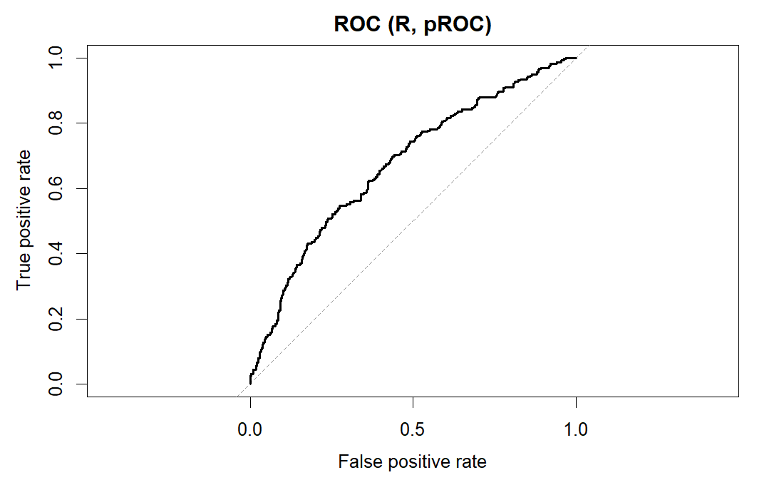
R output. Result:
Area under the curve: 0.6738# OMOP cohort: ROC curve and AUC (discrimination) for a logistic risk model. # cohort.csv, one row per person: age = age in years; sex = sex (M/F); comorbidity = comorbidity count; exposed = drug exposure, 0/1; outcome = outcome condition, 0/1. import matplotlib.pyplot as plt; from sklearn.metrics import roc_curve, roc_auc_score import pandas as pd, statsmodels.formula.api as smf coh = pd.read_csv("https://paulinadelmundomd.com/data/omop/cohort.csv") p = smf.logit("outcome ~ age + C(sex) + comorbidity + exposed", coh).fit(disp=0).predict() fpr, tpr, _ = roc_curve(coh.outcome, p) plt.plot(fpr, tpr, label="Logistic"); plt.plot([0,1],[0,1],"--", label="Chance") plt.xlabel("False positive rate"); plt.ylabel("True positive rate") plt.title("ROC (Python)"); plt.legend() roc_auc_score(coh.outcome, p) # AUC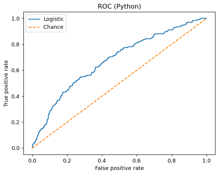
Python output. Result:
0.6738376480148596 - Augmented inverse probability weighting (AIPW)
-
A doubly-robust estimator that corrects an inverse-probability-weighted estimate with a fitted outcome-model term, staying consistent if either the treatment model or the outcome model is right. For \(E[Y(1)]\) it averages \(\mu_1(X_i)+\dfrac{T_i(Y_i-\mu_1(X_i))}{e(X_i)}\), an outcome prediction plus an IPW-weighted residual correction, and equals the sample mean of the efficient influence function. in the pathway → · Tsiatis, 2006
The doubly-robust estimate of the exposure effect is about -0.046 on the risk scale, roughly 4.6 fewer outcomes per 100 exposed after adjustment. It stays consistent as long as either the outcome model or the propensity model is right.
# OMOP cohort: doubly-robust (AIPW) risk difference, PS + outcome models.
# cohort.csv, one row per person: age = age in years; sex = sex (M/F); comorbidity = comorbidity count; exposed = drug exposure, 0/1; outcome = outcome condition, 0/1.
coh <- read.csv("https://paulinadelmundomd.com/data/omop/cohort.csv")
ps <- predict(glm(exposed ~ age + sex + comorbidity, data = coh, family = binomial), type="response")
om <- glm(outcome ~ exposed + age + sex + comorbidity, data = coh, family = binomial)
m1 <- predict(om, transform(coh, exposed=1), type="response")
m0 <- predict(om, transform(coh, exposed=0), type="response")
A <- coh$exposed; Y <- coh$outcome
mean(m1 + A*(Y-m1)/ps) - mean(m0 + (1-A)*(Y-m0)/(1-ps))   # AIPW risk difference
Result:
[1] -0.04576048# OMOP cohort: doubly-robust (AIPW) risk difference, PS + outcome models. # cohort.csv, one row per person: age = age in years; sex = sex (M/F); comorbidity = comorbidity count; exposed = drug exposure, 0/1; outcome = outcome condition, 0/1. import numpy as np, pandas as pd, statsmodels.formula.api as smf coh = pd.read_csv("https://paulinadelmundomd.com/data/omop/cohort.csv") ps = smf.logit("exposed ~ age + C(sex) + comorbidity", coh).fit(disp=0).predict() om = smf.logit("outcome ~ exposed + age + C(sex) + comorbidity", coh).fit(disp=0) m1 = om.predict(coh.assign(exposed=1)); m0 = om.predict(coh.assign(exposed=0)) A, Y = coh.exposed, coh.outcome np.mean(m1 + A*(Y-m1)/ps) - np.mean(m0 + (1-A)*(Y-m0)/(1-ps)) # AIPW risk differenceResult:
-0.045760480970088224 - Autocorrelation
- Correlation of a series with its own past values, so residuals close in time move together. It violates the independence an ordinary regression assumes and, left uncorrected, shrinks standard errors so an effect looks more certain than it is. in the pathway →
B
- Back-door criterion
- A rule for reading an adjustment set off a causal diagram: pick a set of variables that blocks every back-door (non-causal) path between exposure and outcome, meaning every path that runs through a common cause of both. in the pathway →
- Bagging
- Training many trees on bootstrap resamples and averaging them to lower variance, the basis of the random forest. in the pathway →
- Basic reproduction number
- \(R_0\), the average number of secondary cases one infectious person generates in a fully susceptible population, the master number of transmission. \(R_0>1\) lets an epidemic grow and \(R_0<1\) makes it fade; it sets the herd-immunity threshold \(1-1/R_0\) and the final epidemic size. As susceptibles deplete or control bites, the effective reproduction number \(R_t\) falls below \(R_0\), and holding \(R_t<1\) is the aim of control. \(R_0\) is not a fixed property of a pathogen: it depends on contact rates and how long people stay infectious, so it varies by setting. in the pathway → · Dohoo, Martin & Stryhn, 2012
- Bayes factor
- The Bayesian counterpart of a hypothesis test: the ratio of the marginal likelihood of the data under one model to that under another, quantifying how far the data shift the odds between them. Unlike a p-value it can support the null as well as reject it, and it penalises complexity automatically, but it can be highly sensitive to the prior placed on each model’s parameters. Values are read on conventional scales, for instance above 10 as strong evidence. in the pathway → · Dohoo, Martin & Stryhn, 2012 · Kass & Raftery, 1995
- Bayes’ theorem
-
The rule that the posterior is proportional to the likelihood times the prior. in the pathway →
\[\text{posterior} \propto \text{likelihood} \times \text{prior}\]
where \(\text{posterior}\) is the updated distribution of the parameter after seeing the data; \(\text{likelihood}\) is what the data say about the parameter; \(\text{prior}\) is what you believed about the parameter before seeing the data.
Even with 99% sensitivity and 95% specificity, a positive test at 1% prevalence means only a 17% chance of disease: the prior (the base rate) dominates the update, which is exactly the lesson Bayes’ theorem enforces.
# Bayes' theorem as a diagnostic post-test probability: the positive predictive
# value from prevalence P, sensitivity Se, specificity Sp. At low prevalence
# even a very good test yields a low PPV.
P <- 0.01; Se <- 0.99; Sp <- 0.95
Se * P / (Se * P + (1 - Sp) * (1 - P))     # P(disease | test positive)
Result:
[1] 0.1666667# Bayes' theorem as a diagnostic post-test probability: the positive predictive # value from prevalence P, sensitivity Se, specificity Sp. At low prevalence # even a very good test yields a low PPV. P, Se, Sp = 0.01, 0.99, 0.95 Se * P / (Se * P + (1 - Sp) * (1 - P)) # P(disease | test positive)Result:
0.16666666666666655 - Bayesian computation
- Exploring posteriors with no closed form by simulation, principally Markov chain Monte Carlo. in the pathway →
- Bayesian inference
-
Treating the parameter as a random quantity with a distribution the data update, yielding a posterior summarized by a credible interval. in the pathway →
\[p(x,\theta) = p(x \mid \theta)\,p(\theta) = p(\theta \mid x)\,p(x) \;\Rightarrow\; p(\theta \mid x) = \dfrac{p(x \mid \theta)\,p(\theta)}{p(x)} \;\propto\; p(x \mid \theta)\,p(\theta)\]
where \(p(\theta)\) is the prior, \(p(x\mid\theta)\) the likelihood, and \(p(\theta\mid x)\) the posterior. Equating the two factorizations of the joint \(p(x,\theta)\) gives Bayes’ rule; since the evidence \(p(x)\) does not depend on \(\theta\), the posterior is proportional to likelihood times prior.
There is a 95% posterior probability the true event rate lies in [0.265, 0.321]: the direct “the parameter is in here” statement a credible interval licenses and a confidence interval does not.
# Beta-Binomial: a Beta(1, 1) prior updated by the outcome events gives a
# Beta(1 + events, 1 + non-events) posterior; its 2.5th and 97.5th percentiles
# are the 95% credible interval, a direct probability statement about the rate.
# cohort.csv, one row per person: outcome (0/1 event).
coh <- read.csv("https://paulinadelmundomd.com/data/omop/cohort.csv")
k <- sum(coh$outcome); n <- nrow(coh)
qbeta(c(0.025, 0.975), 1 + k, 1 + n - k)   # 95% credible interval for the rate
Result:
[1] 0.2646650 0.3209502# Beta-Binomial: a Beta(1, 1) prior updated by the outcome events gives a # Beta(1 + events, 1 + non-events) posterior; its 2.5th and 97.5th percentiles # are the 95% credible interval, a direct probability statement about the rate. # cohort.csv, one row per person: outcome (0/1 event). import pandas as pd from scipy import stats coh = pd.read_csv("https://paulinadelmundomd.com/data/omop/cohort.csv") k = coh.outcome.sum(); n = len(coh) stats.beta.ppf([0.025, 0.975], 1 + k, 1 + n - k) # 95% credible intervalResult:
array([0.26466504, 0.32095019]) - Belmont principles
- The three principles underpinning research ethics: respect for persons, beneficence, and justice. in the pathway → · HHS OHRP: The Belmont Report ↗
- Benjamini-Hochberg
-
A procedure controlling the false-discovery rate among rejected hypotheses. in the pathway →
\[\text{reject } H_{(i)} \text{ for all } i \le \max\Big\{i : p_{(i)} \le \tfrac{i}{m}\,q\Big\}\]
where \(p_{(i)}\) are the ordered p-values, \(m\) the number of tests, \(q\) the target false-discovery rate.
Three of the four predictors survive FDR control at 5%; n_visits (adjusted p = 0.76) does not. BH is less conservative than Bonferroni because it controls the expected proportion of false discoveries rather than the chance of any.
# OMOP cohort: Benjamini-Hochberg FDR adjustment of the p-values from four
# univariate logistic tests of the outcome, controlling the expected share of
# false positives among the rejections. cohort.csv: outcome and predictors.
coh <- read.csv("https://paulinadelmundomd.com/data/omop/cohort.csv")
vars <- c("age", "comorbidity", "n_visits", "followup_years")
p <- sapply(vars, function(v)
  summary(glm(reformulate(v, "outcome"), binomial, coh))$coef[2, 4])
unname(round(p.adjust(p, "BH"), 4))     # BH-adjusted p-values
Result:
[1] 0.0070 0.0000 0.7621 0.0039# OMOP cohort: Benjamini-Hochberg FDR adjustment of the p-values from four # univariate logistic tests of the outcome, controlling the expected share of # false positives among the rejections. cohort.csv: outcome and predictors. import pandas as pd, statsmodels.formula.api as smf from statsmodels.stats.multitest import multipletests coh = pd.read_csv("https://paulinadelmundomd.com/data/omop/cohort.csv") vars = ["age", "comorbidity", "n_visits", "followup_years"] p = [smf.logit(f"outcome ~ {v}", coh).fit(disp=0).pvalues[v] for v in vars] multipletests(p, method="fdr_bh")[1].round(4).tolist() # BH-adjustedResult:
[0.007, 0.0, 0.7621, 0.0039] - Berkson’s bias
- The spurious association produced by conditioning on hospital admission. in the pathway →
- Best linear unbiased predictor (BLUP)
- The predicted random effects of a mixed model, the BLUPs, estimating each cluster’s departure from the average. They are shrinkage estimates: a group with few observations or weak signal is pulled toward the overall mean, more than its own noisy average would be, borrowing strength across groups in an empirical-Bayes way. This is why mixed-model group estimates are steadier than fitting each group in isolation. in the pathway → · Dohoo, Martin & Stryhn, 2012
- Bias quantification
-
Putting a number on how much unmeasured confounding it would take to overturn a result (for example an E-value, the confounder strength that would explain away the effect). The larger the strength required, the more robust the finding. in the pathway →
The crude risk ratio (0.84, or 1.18 inverted) has an E-value of 1.65: a confounder would need risk-ratio associations of about 1.65 with both exposure and outcome to explain the crude association away fully. That is a modest bar, so the association is not especially robust.
# OMOP cohort: the E-value for the crude exposure-outcome risk ratio, the
# minimum strength (on the risk-ratio scale) an unmeasured confounder would
# need with both exposure and outcome to explain the association away.
# cohort.csv: exposed (0/1), outcome (0/1).
coh <- read.csv("https://paulinadelmundomd.com/data/omop/cohort.csv")
r1 <- mean(coh$outcome[coh$exposed == 1]); r0 <- mean(coh$outcome[coh$exposed == 0])
RR <- r1 / r0; RR <- ifelse(RR < 1, 1 / RR, RR)
RR + sqrt(RR * (RR - 1))   # E-value
Result:
[1] 1.650332# OMOP cohort: the E-value for the crude exposure-outcome risk ratio, the # minimum strength (on the risk-ratio scale) an unmeasured confounder would # need with both exposure and outcome to explain the association away. import pandas as pd, numpy as np coh = pd.read_csv("https://paulinadelmundomd.com/data/omop/cohort.csv") r1 = coh.outcome[coh.exposed == 1].mean(); r0 = coh.outcome[coh.exposed == 0].mean() RR = r1 / r0; RR = 1 / RR if RR < 1 else RR float(RR + np.sqrt(RR * (RR - 1))) # E-valueResult:
1.6503321627308662 - Bias-variance and regularization
- The practical fix for the bias-variance tradeoff: regularization (as in ridge or lasso) deliberately accepts a little bias to cut variance, lowering total prediction error. in the pathway → \[\mathbb{E}\big[(y-\hat f)^{2}\big] = \big(\mathbb{E}[\hat f]-f\big)^{2} + \mathbb{E}\big[(\hat f-\mathbb{E}[\hat f])^{2}\big] + \sigma^{2} = \mathrm{Bias}^{2} + \operatorname{Var} + \sigma^{2}\] where adding and subtracting \(\mathbb{E}[\hat f]\) inside the squared error splits it into squared bias, variance, and the irreducible noise \(\sigma^{2}\); regularization deliberately adds a little bias to cut variance and lower the total.
- Bias-variance tradeoff
- The underlying concept: a too-simple model underfits (high bias) and a too-flexible model overfits (high variance), with prediction error their sum plus irreducible noise. The regularization entry covers how to manage it. in the pathway → \[\text{expected prediction error} = \text{bias}^2 + \text{variance} + \text{irreducible noise}\] where \(\text{expected prediction error}\) is the average error on new data; \(\text{bias}^2\) is the squared error from a model too simple to capture the signal; \(\text{variance}\) is the error from a model flexible enough to chase noise; \(\text{irreducible noise}\) is the variation no model can remove.
- BIC
-
The Bayesian information criterion, like AIC but penalizing each extra parameter more heavily, so it favors smaller models, where lower is better. in the pathway →
\[\mathrm{BIC} = -2\ln \hat L + k\ln n\]
where \(k\) is the number of parameters and \(n\) the sample size.
The comorbidity model wins by about 63 BIC points. Because BIC penalizes parameters by log(n) instead of 2, it favors smaller models than AIC and here reaches the same verdict less generously (the AIC gain was about 68).
# OMOP cohort: BIC, like AIC but with a heavier per-parameter penalty
# (log(n) rather than 2), comparing two logistic models; lower is better.
# cohort.csv: outcome (0/1), age, comorbidity (count).
coh <- read.csv("https://paulinadelmundomd.com/data/omop/cohort.csv")
m1 <- glm(outcome ~ age, binomial, coh)
m2 <- glm(outcome ~ age + comorbidity, binomial, coh)
BIC(m1) - BIC(m2)          # BIC gain from adding comorbidity
Result:
[1] 63.26987# OMOP cohort: BIC, like AIC but with a heavier per-parameter penalty # (log(n) rather than 2), comparing two logistic models; lower is better. import pandas as pd, statsmodels.formula.api as smf coh = pd.read_csv("https://paulinadelmundomd.com/data/omop/cohort.csv") m1 = smf.logit("outcome ~ age", coh).fit(disp=0) m2 = smf.logit("outcome ~ age + comorbidity", coh).fit(disp=0) float(m1.bic - m2.bic) # BIC gain from adding comorbidityResult:
63.26987300102337 - Binomial distribution
-
The distribution of counts of successes. in the pathway → · Dohoo, Martin & Stryhn, 2012
\[P(X=k) = \binom{n}{k} p^{k} (1-p)^{n-k}\]
where \(n\) is the number of independent trials, \(p\) the success probability, and \(k\) the number of successes; the mean is \(np\) and the variance \(np(1-p)\).
With an AE rate near 0.50, exactly 10 of 20 is the single most likely count yet still carries only about 18% probability, because the binomial spreads its mass across every count from 0 to 20.
# CDISC ADaM: the binomial probability of exactly 10 adverse events among 20
# subjects, given the trial's observed per-subject AE rate.
# adsl.csv one row per subject; adae.csv one row per adverse-event record.
adsl <- read.csv("https://paulinadelmundomd.com/data/cdisc/adsl.csv")
adae <- read.csv("https://paulinadelmundomd.com/data/cdisc/adae.csv")
p <- mean(adsl$USUBJID %in% adae$USUBJID)   # per-subject AE rate
dbinom(10, 20, p)          # P(exactly 10 of 20 have an AE)
Result:
[1] 0.1760878# CDISC ADaM: the binomial probability of exactly 10 adverse events among 20 # subjects, given the trial's observed per-subject AE rate. import pandas as pd from scipy import stats adsl = pd.read_csv("https://paulinadelmundomd.com/data/cdisc/adsl.csv") adae = pd.read_csv("https://paulinadelmundomd.com/data/cdisc/adae.csv") p = adsl.USUBJID.isin(adae.USUBJID).mean() # per-subject AE rate float(stats.binom.pmf(10, 20, p)) # P(exactly 10 of 20 have an AE)Result:
0.17608784008487638 - Bivariate tests
-
Classical tests of whether two variables are associated, each a special case of a regression model. in the pathway →
Age differs by outcome status (p = 0.007). Each classical bivariate test, whether t, chi-square, or ANOVA, is a special case of a regression model, so this is the two-variable slice of a model that could then be adjusted.
# OMOP cohort: a Welch two-sample t-test, the classic bivariate test for a
# mean difference, here whether age differs between those with and without
# the outcome. cohort.csv: age, outcome (0/1).
coh <- read.csv("https://paulinadelmundomd.com/data/omop/cohort.csv")
t.test(age ~ outcome, data = coh)$p.value   # H0: equal mean age
Result:
[1] 0.007106646# OMOP cohort: a Welch two-sample t-test, the classic bivariate test for a # mean difference, here whether age differs between those with and without # the outcome. cohort.csv: age, outcome (0/1). import pandas as pd from scipy import stats coh = pd.read_csv("https://paulinadelmundomd.com/data/omop/cohort.csv") a = coh.age[coh.outcome == 1]; b = coh.age[coh.outcome == 0] float(stats.ttest_ind(a, b, equal_var=False).pvalue) # Welch t-testResult:
0.007106645999757379 - Bland-Altman plot
- A plot of differences against means that reveals systematic disagreement two methods can have despite high correlation. in the pathway → · Bland & Altman, 198690837-8)
- Blinding
- Keeping patients, clinicians, and outcome assessors unaware of the assigned arm to prevent the bias that knowing it introduces. in the pathway →
- Block randomization
- Permuted-block randomization that keeps trial arms close to equal in size as enrollment proceeds. in the pathway →
- Bonferroni correction
-
Dividing alpha by the number of tests to control the family-wise error rate. in the pathway →
\[\alpha^{*} = \dfrac{\alpha}{m}\]
where \(m\) is the number of tests; using the smaller threshold \(\alpha^{*}\) for each holds the family-wise error rate at \(\alpha\), at the cost of power.
Under Bonferroni the same tests give larger surviving p-values than BH and push n_visits to 1.0: controlling the chance of any false positive is a stricter bar than controlling their expected fraction.
# OMOP cohort: Bonferroni adjustment of the same four p-values, multiplying
# each by the number of tests (capped at 1) to control the family-wise error
# rate, the chance of even one false positive.
coh <- read.csv("https://paulinadelmundomd.com/data/omop/cohort.csv")
vars <- c("age", "comorbidity", "n_visits", "followup_years")
p <- sapply(vars, function(v)
  summary(glm(reformulate(v, "outcome"), binomial, coh))$coef[2, 4])
unname(round(p.adjust(p, "bonferroni"), 4))   # Bonferroni-adjusted p-values
Result:
[1] 0.0211 0.0000 1.0000 0.0078# OMOP cohort: Bonferroni adjustment of the same four p-values, multiplying # each by the number of tests (capped at 1) to control the family-wise error # rate, the chance of even one false positive. import pandas as pd, statsmodels.formula.api as smf from statsmodels.stats.multitest import multipletests coh = pd.read_csv("https://paulinadelmundomd.com/data/omop/cohort.csv") vars = ["age", "comorbidity", "n_visits", "followup_years"] p = [smf.logit(f"outcome ~ {v}", coh).fit(disp=0).pvalues[v] for v in vars] multipletests(p, method="bonferroni")[1].round(4).tolist() # Bonferroni-adjustedResult:
[0.0211, 0.0, 1.0, 0.0078] - Boosting
- Fitting trees in sequence, each correcting the last’s residuals, to lower bias, as in gradient boosting and XGBoost. in the pathway → \[F_m(x) = F_{m-1}(x) + \gamma_m\, h_m(x)\] where each weak learner \(h_m\) is fit to the current errors, with step size \(\gamma_m\).
- Bootstrap and resampling methods
-
Repeatedly resample the observed data with replacement and recompute the estimate, building an empirical sampling distribution for intervals when analytic standard errors are awkward. in the pathway → · Efron, 1979
The 2.5th to 97.5th percentiles of the resampled means, about 25.1 to 26.1, form a 95% CI for mean BMI without assuming normality. A wider interval would signal a less stable estimate.
# CDISC ADaM ADSL: bootstrap 95% CI for the mean baseline BMI.
# adsl.csv, one row per subject: BMIBL = baseline BMI.
set.seed(1); adsl <- read.csv("https://paulinadelmundomd.com/data/cdisc/adsl.csv")
bs <- replicate(2000, mean(sample(adsl$BMIBL, replace = TRUE)))
quantile(bs, c(.025, .975))   # percentile bootstrap CI
Result:
    2.5%    97.5%
25.12508 26.07131
# CDISC ADaM ADSL: bootstrap 95% CI for the mean baseline BMI. # adsl.csv, one row per subject. import numpy as np, pandas as pd rng = np.random.default_rng(1); x = pd.read_csv("https://paulinadelmundomd.com/data/cdisc/adsl.csv").BMIBL.values bs = [rng.choice(x, x.size, replace=True).mean() for _ in range(2000)] np.percentile(bs, [2.5, 97.5]) # percentile bootstrap CIResult:
[25.11689961 26.03783465] - Bradford Hill viewpoints
- The nine considerations (temporality, strength, consistency, biological gradient, plausibility, coherence, experiment, specificity, analogy) used to weigh whether an observed association should be read as causal. They are viewpoints to weigh rather than a checklist to count: only temporality is necessary, and they organize the argument that an explicit estimand, a causal diagram, and quantified bias then have to make rigorous. in the pathway →
- Brier score
-
The mean squared difference between predicted probabilities and binary outcomes, a proper scoring rule that rewards both calibration and discrimination; lower is better. in the pathway → · Brier, 1950
The mean squared gap between predicted risk and outcome is 0.19. Lower is better; 0 is perfect and 0.25 is what you get by predicting 0.5 for everyone, so 0.19 is only modestly better than uninformative.
# OMOP cohort: Brier score (mean squared error of predicted risks).
# cohort.csv, one row per person: age = age in years; sex = sex (M/F); comorbidity = comorbidity count; exposed = drug exposure, 0/1; outcome = outcome condition, 0/1.
coh <- read.csv("https://paulinadelmundomd.com/data/omop/cohort.csv")
p <- predict(glm(outcome ~ age + sex + comorbidity + exposed, coh, family=binomial), type="response")
mean((p - coh$outcome)^2)   # lower is better
Result:
[1] 0.1903675# OMOP cohort: Brier score (mean squared error of predicted risks). # cohort.csv, one row per person: age = age in years; sex = sex (M/F); comorbidity = comorbidity count; exposed = drug exposure, 0/1; outcome = outcome condition, 0/1. from sklearn.metrics import brier_score_loss import pandas as pd, statsmodels.formula.api as smf coh = pd.read_csv("https://paulinadelmundomd.com/data/omop/cohort.csv") p = smf.logit("outcome ~ age + C(sex) + comorbidity + exposed", coh).fit(disp=0).predict() brier_score_loss(coh.outcome, p) # lower is betterResult:
0.19036752738691223 - Budget impact analysis
- Projecting the total cost to a specific budget holder of adopting an intervention across the eligible population over a near-term horizon under realistic uptake. in the pathway →
C
- Calibration
- Whether a model’s predicted risks match observed event rates, read off a calibration plot or tested with goodness-of-fit. in the pathway →
- Calibration (modeling)
- In a decision or simulation model, tuning an unobservable input until the model’s outputs match observed targets (such as known survival or prevalence), with the resulting uncertainty carried forward. This is distinct from the prediction-model sense of whether predicted risks match observed rates. in the pathway →
- Calibration versus discrimination
-
Discrimination asks whether a model ranks higher-risk patients above lower-risk ones, while calibration asks whether predicted risks match observed rates. in the pathway →
Points on the 45-degree line mean predicted risk matches observed frequency, which is good calibration. Discrimination is a separate property (the AUC); a model can rank cases well yet be miscalibrated, or the reverse.
# OMOP cohort: calibration plot (predicted vs observed risk by decile).
# cohort.csv, one row per person: age = age in years; sex = sex (M/F); comorbidity = comorbidity count; exposed = drug exposure, 0/1; outcome = outcome condition, 0/1.
coh <- read.csv("https://paulinadelmundomd.com/data/omop/cohort.csv")
p <- predict(glm(outcome ~ age + sex + comorbidity + exposed, coh, family=binomial), type="response")
g <- cut(p, quantile(p, 0:10/10), include.lowest=TRUE)
plot(tapply(p, g, mean), tapply(coh$outcome, g, mean), pch=16,
     xlab="Predicted risk", ylab="Observed risk", main="Calibration (R)"); abline(0, 1, lty=2)
invisible()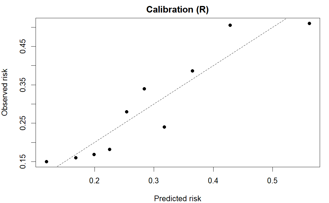
R output. # OMOP cohort: calibration plot (predicted vs observed risk by decile). # cohort.csv, one row per person: age = age in years; sex = sex (M/F); comorbidity = comorbidity count; exposed = drug exposure, 0/1; outcome = outcome condition, 0/1. import matplotlib.pyplot as plt; from sklearn.calibration import calibration_curve import pandas as pd, statsmodels.formula.api as smf coh = pd.read_csv("https://paulinadelmundomd.com/data/omop/cohort.csv") p = smf.logit("outcome ~ age + C(sex) + comorbidity + exposed", coh).fit(disp=0).predict() obs, pred = calibration_curve(coh.outcome, p, n_bins=10) plt.plot(pred, obs, "o-"); plt.plot([0,1],[0,1],"--") plt.xlabel("Predicted risk"); plt.ylabel("Observed risk"); plt.title("Calibration (Python)") plt.show()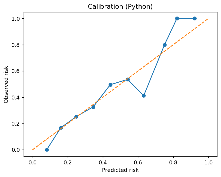
Python output. - Case definition
- The explicit criteria a person must meet to be counted as a case. A clear, consistently applied case definition, backed by surveillance able to find all such cases, is what makes any frequency measure reliable and comparable across studies. in the pathway → · Dohoo, Martin & Stryhn, 2012
- Case fatality rate
- The share of people with a disease who die of it within a defined period, \(\text{CFR} = \text{deaths}/\text{cases}\). Despite the name it is a risk, a proportion, not a true rate; it measures how deadly a disease is for those who contract it. It is common in outbreak and acute-disease reporting. in the pathway → · Dohoo, Martin & Stryhn, 2012
- Case report
- A description of a single patient or a handful, usually a rare condition or an unusual presentation of a common one. It has no comparison group and so can support no claim about cause, but the oddity it records is often what first suggests a hypothesis worth testing in an analytic study. in the pathway → · Dohoo, Martin & Stryhn, 2012
- Case series
- A description of the occurrence or clinical course of a condition across a group of patients, documenting who was affected, when, and where. Like a case report it has no comparison group, so it cannot measure an association; it can describe prognosis if the cases are representative, and it generates hypotheses rather than testing them. Distinct from the self-controlled case series, which is an analytic design. in the pathway → · Dohoo, Martin & Stryhn, 2012
- Case-case study
- A case-control variant whose controls are subjects with a related but distinct disease, such as a different serovar of the same pathogen drawn from the same surveillance system. Because cases and control-cases share the selection and reporting experience, it curbs selection and recall bias and needs no separate control group, which helps for reportable-disease data where valid controls are hard to define. Its cost is interpretive: the control-cases’ exposure does not estimate exposure in the source population, so the odds ratio contrasts two disease subtypes rather than measuring risk, and risk factors the subtypes share cannot be found. Best suited to short-induction exposures such as food-borne pathogens. in the pathway → · Dohoo, Martin & Stryhn, 2012
- Case-case-control study
- A case-control design with two distinct case series and one shared control series, developed to separate risk factors for antimicrobial resistance, for example vancomycin-resistant versus susceptible Enterococcus. Each case series is modelled separately against the common controls by logistic regression: a factor appearing only in the resistant model is a resistance-specific risk factor, only in the susceptible model a susceptibility-specific one, and in both a risk factor for the organism in general. It is argued to be more valid than a direct case-case comparison when resistance is acquired from outside rather than emerging de novo. in the pathway → · Dohoo, Martin & Stryhn, 2012
- Case-cohort design
- Samples a random subcohort plus all cases, letting one comparison group serve several outcomes from the same source population. in the pathway →
- Case-cohort study
- A cohort design that measures expensive exposures on only a random subcohort drawn at baseline plus every case arising in the full cohort, buying cohort validity at case-control cost. One subcohort can serve as the comparison for several outcomes at once, and because it is a random sample of the base it can also estimate disease frequency. A closed population allows a risk-based odds ratio analysis; an open one uses Cox regression with weights inverse to the sampling probability (Prentice’s method) and robust standard errors. It differs from the nested case-control study, whose controls are re-sampled at each case’s event time rather than fixed as one subcohort. in the pathway → · Dohoo, Martin & Stryhn, 2012
- Case-control study
- Starts from outcome status, comparing prior exposure in cases versus controls; efficient for rare outcomes and long latencies. in the pathway → · Dohoo, Martin & Stryhn, 2012
- Case-crossover design
- A self-controlled case-control variant in which each case is its own control: exposure in the short window just before the event is compared with the same person’s exposure in earlier or later reference windows, so every time-invariant confounder is controlled by design. It answers the ‘why now’ rather than the ‘why me’ question, and suits transient triggers of abrupt outcomes such as air pollution or acute injury. Reference windows are placed symmetrically around the event (bidirectional) or time-stratified so exposure trends cancel, and the design assumes no trend in exposure across the window and that the event does not change later exposure. Analyse as matched data with McNemar’s test or conditional logistic regression. in the pathway → · Dohoo, Martin & Stryhn, 2012
- Case-only study
- A design that uses cases alone to estimate an exposure-by-covariate interaction, not main effects, when exposure and covariate can be assumed independent in the source population; its original use was gene-environment interaction, where the control genotype distribution is known on theoretical grounds. Among cases, a logistic model of the covariate on the exposure, \(\operatorname{logit}\Pr(\text{covariate}=1)=\beta_0+\beta_1\,\text{exposure}\), returns a \(\beta_1\) equal to the interaction term of the full Poisson model. It is highly efficient since no controls are gathered, but the independence assumption is strong and biases the estimate when it fails, and it speaks only to effect modification, never to the exposure’s main effect. in the pathway → · Dohoo, Martin & Stryhn, 2012
- Case-time-control design
- Adds a control group to the case-crossover design to adjust for exposure trends over calendar time. in the pathway →
- Categorizing continuous variables
- Cutting a continuous predictor into categories (tertiles, a clinical threshold) before modelling. It eases interpretation and can hint at a nonlinear shape, but it discards information, so it loses power, can leave residual confounding within broad bands, and makes results sensitive to where the cut-points land. Keeping the variable continuous, with splines or fractional polynomials for curvature, is generally preferred. in the pathway → · Dohoo, Martin & Stryhn, 2012
- Causal complement
- In the sufficient-component cause model, the set of co-factors that must join an exposure to complete a sufficient cause (a complete set of conditions that together guarantee disease). Because an exposure only produces disease when its causal complement is present, how common those co-factors are in a population sets the measured strength of association, not the biology alone. in the pathway → · Dohoo, Martin & Stryhn, 2012
- Causal designs without randomization
- A set of designs, each neutralizing a specific dominant threat to causal inference, matched to the threat endangering the question. Examples include difference-in-differences, regression discontinuity, and instrumental variables. in the pathway →
- Causal diagrams
- A directed acyclic graph of assumed causal effects that sorts each covariate into a confounder, mediator, or collider. in the pathway → · Dohoo, Martin & Stryhn, 2012
- Causal estimators
- Methods that compute the effect once the design and the set of confounders to adjust for are chosen, including propensity scores and g-methods (a family of methods built for treatments and confounders that change over time). in the pathway →
- Cause-specific hazard
- Instantaneous event rate among patients still at risk, used to study etiology and biological mechanism. in the pathway → \[h_k(t) = \lim_{\Delta t \to 0}\dfrac{P(t \le T < t+\Delta t,\ D=k \mid T \ge t)}{\Delta t}\] where \(D=k\) denotes failure from cause \(k\) among those still at risk.
- Cause-specific mortality rate
- The mortality rate restricted to deaths from (or with) one specific disease, per unit of person-time. Its denominator is the whole population, which distinguishes it from the case fatality rate, whose denominator is only the cases. in the pathway → · Dohoo, Martin & Stryhn, 2012
- CDISC SDTM
- The Study Data Tabulation Model, a Clinical Data Interchange Standards Consortium (CDISC) standard for structuring clinical trial tabulation data. in the pathway → · CDISC SDTM ↗
- Censoring
- When a subject’s event time is known only to exceed their observed follow-up, as when they are still event-free at study end or lost to follow-up. Survival methods handle it by crediting each subject their time at risk; the danger is informative censoring, where the reason for leaving is tied to the outcome, which biases the estimate much as selection does. Distinct from a competing risk, which removes the possibility of the event entirely. in the pathway → · Rothman, Greenland & Lash, 2008
- Central limit theorem
-
The result that the mean of a large enough sample is approximately normal whatever the underlying shape, enabling z- and t-based inference. in the pathway →
\[\bar{X} \;\approx\; N\!\left(\mu,\ \dfrac{\sigma^2}{n}\right)\]
where for a large sample of size \(n\), the sampling distribution of the mean \(\bar{X}\) is approximately normal regardless of the shape of the underlying data, with standard error \(\sigma/\sqrt{n}\).
The mean age is pinned to within a standard error of about 0.51 years. The CLT is what lets a normal-based confidence interval attach to that mean without assuming age itself is normal, given a large enough n.
# OMOP cohort: the central limit theorem says the sample mean is approximately
# normal with standard error SD/sqrt(n), whatever age's own shape. cohort.csv: age.
coh <- read.csv("https://paulinadelmundomd.com/data/omop/cohort.csv")
sd(coh$age) / sqrt(nrow(coh))    # standard error of the mean age
Result:
[1] 0.5053451# OMOP cohort: the central limit theorem says the sample mean is approximately # normal with standard error SD/sqrt(n), whatever age's own shape. cohort.csv: age. import pandas as pd, numpy as np coh = pd.read_csv("https://paulinadelmundomd.com/data/omop/cohort.csv") float(coh.age.std(ddof=1) / np.sqrt(len(coh))) # standard error of the mean ageResult:
0.5053450876951884 - Certainty of evidence (GRADE)
- Rating how much confidence a body of evidence warrants, separately from effect size, downgrading for risk of bias, inconsistency, indirectness, imprecision, and publication bias. in the pathway → · GRADE working group ↗
- Change-in-estimate
-
The workhorse rule for spotting a confounder: add the candidate to the model and see whether the exposure’s effect estimate shifts materially, a common threshold being a 10% change in the odds ratio or coefficient. A meaningful move means the variable was mixing its effect into the association and should be kept; a negligible move means little confounding by it. Unlike a significance test on the covariate, it targets bias in the estimate of interest rather than the covariate’s own p-value, and it misleads when the variable is a mediator or collider. in the pathway → · Dohoo, Martin & Stryhn, 2012
Adjusting moves the exposure OR by only about 2%, well under the customary 10% flag, so these covariates are not meaningfully confounding the association. The rule swaps a hypothesis test for a direct look at how much the estimate shifts.
# OMOP cohort: the change-in-estimate rule for confounding -- how much the
# exposure odds ratio moves when covariates are added; a large shift flags
# confounding. cohort.csv: outcome, exposed, age, comorbidity, n_visits.
coh <- read.csv("https://paulinadelmundomd.com/data/omop/cohort.csv")
or_crude <- exp(coef(glm(outcome ~ exposed, binomial, coh))["exposed"])
or_adj <- exp(coef(glm(outcome ~ exposed + age + comorbidity + n_visits, binomial, coh))["exposed"])
unname((or_crude - or_adj) / or_adj * 100)   # % change in the OR
Result:
[1] -2.352118# OMOP cohort: the change-in-estimate rule for confounding -- how much the # exposure odds ratio moves when covariates are added; a large shift flags # confounding. cohort.csv: outcome, exposed, age, comorbidity, n_visits. import pandas as pd, numpy as np, statsmodels.formula.api as smf coh = pd.read_csv("https://paulinadelmundomd.com/data/omop/cohort.csv") or_crude = np.exp(smf.logit("outcome ~ exposed", coh).fit(disp=0).params["exposed"]) or_adj = np.exp(smf.logit("outcome ~ exposed + age + comorbidity + n_visits", coh).fit(disp=0).params["exposed"]) float((or_crude - or_adj) / or_adj * 100) # % change in the ORResult:
-2.352118135219176 - Charlson comorbidity index (CCI)
- A weighted count of selected serious conditions, originally calibrated to predict one-year mortality, used as a single comorbidity summary. in the pathway → · Charlson et al., 1987 \[\text{CCI} = \sum_i w_i\, x_i\] where \(x_i\) indicates the presence of condition \(i\) in the lookback window and \(w_i\) its assigned weight (1 to 6); the weighted sum predicts mortality risk.
- CHEERS
- Consolidated Health Economic Evaluation Reporting Standards, the reporting checklist for economic evaluations, the economic-evaluation member of the reporting-standards family. in the pathway → · CHEERS statement (EQUATOR) ↗
- Chi-square test
-
A test of independence between two categorical variables, \(\chi^2 = \sum \dfrac{(\text{obs}-\text{exp})^2}{\text{exp}}\), where each cell’s expected count is its row total times its column total over the grand total. It needs every expected count above 1 and most above 5, with Fisher’s exact test used when counts are small. The Mantel-Haenszel version differs only by a factor of \(n/(n-1)\) and is the one usually applied to stratified data. in the pathway → · Dohoo, Martin & Stryhn, 2012
\[\chi^2 = \sum \dfrac{(O - E)^2}{E}\]
where \(O\) are observed and \(E\) expected cell counts under independence; large values indicate association between two categorical variables.
p below 0.001 means the disease proportion is not independent of arm, so the association is larger than chance would give. Chi-square tests only whether an association exists, not its size or direction.
# CDISC ADaM: chi-square test of dizziness (an AE) against treatment arm.
# adsl.csv, one row per subject: USUBJID = subject id linking the tables; TRT01P = planned arm.
# adae.csv, one row per adverse-event record: AEDECOD = adverse-event term.
adsl <- read.csv("https://paulinadelmundomd.com/data/cdisc/adsl.csv"); adae <- read.csv("https://paulinadelmundomd.com/data/cdisc/adae.csv")
adsl$dz <- as.integer(adsl$USUBJID %in% adae$USUBJID[adae$AEDECOD == "DIZZINESS"])
chisq.test(table(adsl$TRT01P, adsl$dz))
Result:
    Pearson's Chi-squared test

data:  table(adsl$TRT01P, adsl$dz)
X-squared = 14.855, df = 2, p-value = 0.0005947
# CDISC ADaM: chi-square test of dizziness (an AE) against treatment arm. # adsl.csv, one row per subject. # adae.csv, one row per adverse-event record. import pandas as pd; from scipy.stats import chi2_contingency adsl = pd.read_csv("https://paulinadelmundomd.com/data/cdisc/adsl.csv"); adae = pd.read_csv("https://paulinadelmundomd.com/data/cdisc/adae.csv") adsl["dz"] = adsl.USUBJID.isin(adae.USUBJID[adae.AEDECOD == "DIZZINESS"]).astype(int) chi2_contingency(pd.crosstab(adsl.TRT01P, adsl.dz))Result:
Chi2ContingencyResult(statistic=np.float64(14.854858473147846), pvalue=np.float64(0.0005947144184846745), dof=2, expected_freq=array([[80.78740157, 14.21259843], [74.83464567, 13.16535433], [60.37795276, 10.62204724]])) - Choropleth map
- A thematic map that shades geographic areas (counties, census tracts) by the value of a variable such as a disease rate, the standard tool of disease mapping. It is easy to read but can mislead: large, sparsely populated areas dominate the eye, rates in small-population areas are unstable, and the impression shifts with how the values are binned into colour classes. Rate smoothing or mapping a model-based estimate tempers the instability. in the pathway → · Dohoo, Martin & Stryhn, 2012
- Claims and coding standards
- The coded vocabularies behind each claim field, where analysis depends on knowing what each captures and how they map to one another. in the pathway →
- Claims data
- Billing-driven encounter and prescription data covering a payer’s population broadly, where a code is a bill not a diagnosis and clinical detail is thin. in the pathway →
- Claims-based frailty index
- A frailty proxy built from diagnosis and service codes, approximating functional decline when direct frailty assessment is unavailable in data. in the pathway →
- Claims/EHR phenotype algorithm
- A rule mapping recorded codes and encounters to a presumed clinical event or condition. in the pathway →
- Classification performance metrics
- Measures read off the confusion matrix of predicted versus actual, including precision, recall, and F1. in the pathway → \[F_1 = \dfrac{2\,\text{precision}\cdot\text{recall}}{\text{precision}+\text{recall}}\] where the harmonic mean of precision and recall, read off the confusion matrix.
- Clinical equipoise
- Genuine uncertainty in the expert community about which trial arm is better, the ethical license to randomize patients. in the pathway →
- Clinical trial phases
- The staged sequence of pre-marketing drug evaluation. Phase 0 gives a subtherapeutic microdose to a handful of subjects to check that human pharmacokinetics match preclinical predictions; Phase I tests safety and pharmacodynamics in 20-100 healthy volunteers; Phase II first gauges efficacy and dose in 100-300 patients (often a case series or small RCT); Phase III is the large confirmatory RCT, hundreds to thousands, against the standard of care; and Phase IV is post-marketing surveillance for long-term and rare harms. Each phase gates the next, and Phase II results predict Phase III success only weakly. in the pathway → · Dohoo, Martin & Stryhn, 2012
- Clone-censor-weight
- A per-protocol target-trial method that clones patients into each strategy, censors deviators, and reweights to avoid immortal time bias. in the pathway →
- Closed population
- A population with no additions and few or no losses over the study period, so members can in principle be followed for the full risk period; it is the setting in which a risk can be computed directly. Losses that do occur are withdrawals. in the pathway → · Dohoo, Martin & Stryhn, 2012
- Closed question
- A question answered by choosing from a fixed list, easier to answer and to code than an open question. Common forms are the checklist (check all that apply, each option its own 0/1 variable), the two-choice or multiple-choice question (options should be mutually exclusive and exhaustive, with an ‘Other, please specify’ as a semi-open catch-all), the rating question (see Likert scale), and the ranking question. The cost is that a fixed list can oversimplify, or draw an answer where no real opinion exists. in the pathway → · Dohoo, Martin & Stryhn, 2012
- Cluster sampling
- Drawing whole groups such as schools or blocks to cut field cost when no list of individuals exists. in the pathway → · Dohoo, Martin & Stryhn, 2012
- Cluster-randomized trial
- A trial that randomizes groups (clinics, schools, villages) rather than individuals, used when the intervention is delivered at the group level; its correlated outcomes force a design-effect inflation of the sample size. in the pathway →
- Cluster-robust standard errors
- Standard errors that widen a model’s intervals to account for correlation within clusters, leaving the point estimate and the model unchanged; the cheapest way to keep inference honest under clustering. in the pathway →
- Clustered and longitudinal data
- Data whose rows are not independent because observations group within clusters (patients within hospitals) or repeat within a unit over time; the within-cluster correlation means the data carry less information than their count suggests, so ignoring it makes standard errors too small. in the pathway →
- Clustering
- Grouping similar observations, used for phenotyping disease subtypes from a panel of measurements. in the pathway →
- Cochran’s Q
-
A statistical test for heterogeneity across studies in a meta-analysis. in the pathway →
\[Q = \sum_i w_i (y_i - \bar{y})^2\]
where \(w_i\) are inverse-variance weights, \(y_i\) the study effects, and \(\bar{y}\) the pooled effect; under homogeneity \(Q\) follows a chi-square with \(k-1\) degrees of freedom for \(k\) studies.
Cochran’s Q of 37.8 on 11 degrees of freedom (p < 0.001) sits far above its degrees of freedom, so the studies’ effects vary more than sampling error alone would produce: real heterogeneity is present. Q underlies I-squared and tau-squared, though with few studies it can miss heterogeneity, so it is read alongside them.
# Cochran's Q: weighted sum of squared deviations from the fixed-effect mean.
# studies.csv, one row per trial in a meta-analysis: yi = effect estimate, log odds ratio; sei = standard error of yi.
library(metafor)
d <- read.csv("https://paulinadelmundomd.com/data/meta/studies.csv")
res <- rma(yi, sei = sei, data = d)
c(Q = res$QE, df = res$k - 1, p = res$QEp)
Result:
           Q           df            p
3.780392e+01 1.100000e+01 8.442631e-05
# studies.csv, one row per trial in a meta-analysis: yi = effect estimate, log odds ratio. import numpy as np, pandas as pd d = pd.read_csv("https://paulinadelmundomd.com/data/meta/studies.csv") yi = d.yi.values; vi = d.sei.values**2; k = len(yi); w = 1/vi Q = (w*(yi - (w*yi).sum()/w.sum())**2).sum() tau2 = max(0, (Q-(k-1)) / (w.sum() - (w**2).sum()/w.sum())) wr = 1/(vi+tau2); mu = (wr*yi).sum()/wr.sum(); se = wr.sum()**-0.5 from scipy.stats import chi2 print("Q=%.2f df=%d p=%.3f" % (Q, k-1, chi2.sf(Q, k-1)))Result:
Q=37.80 df=11 p=0.000 - Code crosswalks and mappings
- Lookup tables translating one vocabulary into another, each translation lossy in known ways. in the pathway →
- Coefficient of variation
-
A unitless measure of relative variability, the standard deviation divided by the mean, \(\text{CV} = \sigma/\mu\). Used to summarize the precision of a quantitative assay, it lets variability be compared across measurements made on different scales. in the pathway → · Dohoo, Martin & Stryhn, 2012
Age has a CV of 0.26: its standard deviation is about a quarter of its mean. Being unitless, the CV compares variability across quantities on different scales, which the raw SD cannot.
# OMOP cohort: coefficient of variation of age, a unitless measure of relative
# spread (SD / mean). cohort.csv: age.
coh <- read.csv("https://paulinadelmundomd.com/data/omop/cohort.csv")
sd(coh$age) / mean(coh$age)     # CV of age
Result:
[1] 0.2613143# OMOP cohort: coefficient of variation of age, a unitless measure of relative # spread (SD / mean). cohort.csv: age. import pandas as pd coh = pd.read_csv("https://paulinadelmundomd.com/data/omop/cohort.csv") float(coh.age.std(ddof=1) / coh.age.mean()) # CV of ageResult:
0.26131430184359566 - Cohen’s d
-
The effect-size measure accompanying a t-test. in the pathway →
\[d = \dfrac{\bar{X}_1 - \bar{X}_2}{s_{\text{pooled}}}\]
where the mean difference in pooled standard deviation units; a scale-free effect size (about 0.2 small, 0.5 medium, 0.8 large).
d = 0.20 is a small effect by convention: the group means differ by about a fifth of a standard deviation. Where the t-test says whether a difference is detectable, d says how big it is.
# OMOP cohort: Cohen's d, the standardized mean difference in age between those
# with and without the outcome (mean difference / pooled SD). cohort.csv: age, outcome.
coh <- read.csv("https://paulinadelmundomd.com/data/omop/cohort.csv")
g1 <- coh$age[coh$outcome == 1]; g0 <- coh$age[coh$outcome == 0]
sp <- sqrt(((length(g1)-1)*var(g1) + (length(g0)-1)*var(g0)) / (length(g1)+length(g0)-2))
(mean(g1) - mean(g0)) / sp      # Cohen's d
Result:
[1] 0.1956141# OMOP cohort: Cohen's d, the standardized mean difference in age between those # with and without the outcome (mean difference / pooled SD). cohort.csv: age, outcome. import pandas as pd, numpy as np coh = pd.read_csv("https://paulinadelmundomd.com/data/omop/cohort.csv") g1 = coh.age[coh.outcome == 1]; g0 = coh.age[coh.outcome == 0] sp = np.sqrt(((len(g1)-1)*g1.var(ddof=1) + (len(g0)-1)*g0.var(ddof=1)) / (len(g1)+len(g0)-2)) float((g1.mean() - g0.mean()) / sp) # Cohen's dResult:
0.1956141494902175 - Cohen’s kappa
-
A measure of two raters’ categorical agreement corrected for what chance alone would produce, \(\kappa = (p_o - p_e)/(1 - p_e)\) with \(p_o\) the observed and \(p_e\) the chance agreement; it runs from 0 (chance) to 1 (perfect) and is depressed at very high or very low prevalence. in the pathway → · Cohen, 1960
\[\kappa = \frac{p_o - p_e}{1 - p_e}\]
where \(\kappa\) is Cohen’s kappa, the chance-corrected agreement; \(p_o\) is the observed agreement between the two raters; \(p_e\) is the agreement expected if the raters labelled independently.
Raw agreement is 85%, but chance alone would give about 50%, so kappa discounts it to 0.70 (substantial). Kappa can look poor when one category is rare even if raters mostly agree, so it is read next to the raw percentage.
# Cohen's kappa for two raters classifying the same items, corrected for chance
# agreement: kappa = (p_o - p_e) / (1 - p_e). Worked on a 2x2 agreement table
# (both positive 40, both negative 45, 15 disagreements).
tab <- matrix(c(40, 10, 5, 45), 2, 2, byrow = TRUE); N <- sum(tab)
po <- sum(diag(tab)) / N
pe <- sum(rowSums(tab) * colSums(tab)) / N^2
(po - pe) / (1 - pe)            # chance-corrected agreement
Result:
[1] 0.7# Cohen's kappa for two raters classifying the same items, corrected for chance # agreement: kappa = (p_o - p_e) / (1 - p_e). Worked on a 2x2 agreement table # (both positive 40, both negative 45, 15 disagreements). import numpy as np tab = np.array([[40, 10], [5, 45]]); N = tab.sum() po = np.trace(tab) / N pe = (tab.sum(1) @ tab.sum(0)) / N**2 float((po - pe) / (1 - pe)) # chance-corrected agreementResult:
0.7 - Cohort study
- Follows defined people forward from exposure to outcome; prospective when assembled before outcomes occur, retrospective when reconstructed from existing records. It can be built as two cohorts chosen by known exposure status, or as a single cohort (a longitudinal study) sampled where exposure is expected to vary and sorted out afterwards. Whether it is risk-based or rate-based follows from the risk period and whether the population is closed. in the pathway → · Dohoo, Martin & Stryhn, 2012
- Collapsibility
- Whether a marginal effect equals a weighted average of the stratum-specific effects; the risk ratio and risk difference are collapsible, the odds ratio and hazard ratio are not, so the latter can shift on adjustment even without confounding. in the pathway →
- Collider
- A common effect of two variables, where adjusting actively opens bias rather than removing it. in the pathway → · Dohoo, Martin & Stryhn, 2012
- Comorbidity and frailty adjustment
- Summarizing a patient’s baseline illness burden from claims into a validated score used to adjust for confounding by underlying health. in the pathway →
- Comparative effectiveness research
- Research comparing the real-world effects of treatments or procedures on clinical outcomes, as against establishing efficacy versus placebo under trial conditions. It leans heavily on observational data, which is why its credibility rests on design discipline, ideally emulating a target trial, rather than on the analysis alone. in the pathway → · Dohoo, Martin & Stryhn, 2012
- Compartmental model
- A mechanistic transmission model that sorts a population into compartments by infection state, most simply Susceptible-Infectious-Recovered (SIR), with differential equations for the flows between them. SEIR adds an Exposed (latent) stage; further compartments capture waning immunity, vaccination, or age structure. Such models produce an epidemic curve, estimate \(R_0\), and let analysts try interventions in silico, at the cost of strong assumptions about mixing and parameters. in the pathway → · Dohoo, Martin & Stryhn, 2012
- Competing risks
- A setting where one event, such as death, prevents the event of interest from ever occurring. in the pathway → \[F_k(t) = \int_0^t S(u^-)\,h_k(u)\,du\] where \(F_k\) is the cumulative incidence of cause \(k\), \(h_k\) its cause-specific hazard, and \(S\) the overall (all-cause) survival just before \(u\).
- Competing risks and survival models
- Methods for time-to-event data where competing events block the outcome or where parametric forms replace the proportional hazards assumption. in the pathway →
- Complete-case analysis
- Restricting the analysis to records with no missing values, unbiased only under MCAR and otherwise discarding information and risking a distorted estimate. in the pathway →
- Complex-sample design and survey weighting
-
Design-aware analysis using survey weights, strata, and primary sampling units so an oversampled, clustered sample speaks for its population. in the pathway → · Dohoo, Martin & Stryhn, 2012
Weighting shifts the estimate (0.41 against 0.32 unweighted) because the higher-prevalence regions were under-sampled and so carry larger weights. The design-based SE (0.031) runs about twice the naive one (0.015), and that gap is the design effect, \((0.031/0.015)^2 \approx 4.5\): the clustered sample of 990 carries only about the information of 220 independent observations.
# A synthetic complex survey: regions (strata) -> communities (PSUs) -> people,
# with unequal weights and a clustered binary outcome. Columns: stratum, psu, weight, y (0/1).
library(survey)
d <- read.csv("https://paulinadelmundomd.com/data/survey/complex_survey.csv")
des <- svydesign(ids = ~psu, strata = ~stratum, weights = ~weight, data = d, nest = TRUE)
svymean(~y, des)                             # weighted prevalence + design-based SE
sqrt(mean(d$y) * (1 - mean(d$y)) / nrow(d))  # naive SRS SE, ignoring the design
Result:
    mean     SE
y 0.4074 0.0314
[1] 0.01486482
# Same design-based estimate by Taylor linearization, no survey package needed. import pandas as pd, numpy as np d = pd.read_csv("https://paulinadelmundomd.com/data/survey/complex_survey.csv") phat = np.average(d.y, weights=d.weight) # weighted (Hajek) prevalence d["z"] = d.weight * (d.y - phat) / d.weight.sum() # Taylor-linearized residual psu = d.groupby(["stratum", "psu"]).z.sum().reset_index() # PSU totals within strata var = psu.groupby("stratum").z.apply( # stratified between-PSU variance lambda t: len(t) / (len(t) - 1) * ((t - t.mean())**2).sum()).sum() se = np.sqrt(var) # design-based SE round(phat, 4), round(se, 4), round(np.sqrt(d.y.mean() * (1 - d.y.mean()) / len(d)), 4)Result:
(0.4074, 0.0314, 0.0149) - Component cause
- One factor within a sufficient cause (a complete set of conditions that together guarantee disease); the components may act together or in sequence, and a single factor can belong to several distinct sufficient causes. in the pathway → · Dohoo, Martin & Stryhn, 2012
- Composite endpoint
- A single outcome built by combining several events, such as death, myocardial infarction, and stroke, so that any one of them counts, raising the event rate and the trial’s power. The danger is that a large effect on a minor but frequent component can carry the composite while the serious components are unmoved, so the components should be of comparable importance and always reported separately. Distinct from a surrogate endpoint, which substitutes a marker for the clinical outcome rather than bundling outcomes together. in the pathway → · Dohoo, Martin & Stryhn, 2012
- Composite reference standard
- (CRS) A stand-in for a missing gold standard: several imperfect tests are combined by a rule fixed in advance (often, reference-negative samples are re-tested with a resolver and anyone positive on either is called positive), and the new test is judged against that composite. Unlike discrepant resolution, which re-tests only the disagreements and so biases the result toward the index test, a CRS is defined without reference to the test being evaluated. in the pathway → · Dohoo, Martin & Stryhn, 2012
- Composite strategy
- An intercurrent-event strategy that folds the event into the endpoint. in the pathway →
- Concordance correlation coefficient
-
- A measure of agreement between two continuous measurements that rewards falling on the 45-degree line of perfect concordance, not merely being linearly related. It multiplies a Pearson correlation (how tight the scatter) by an accuracy term (how far the fitted line sits from the diagonal in shift and slope); 1 is perfect agreement. Preferred over a plain Pearson correlation, which ignores systematic shifts, and complementary to a Bland-Altman plot. in the pathway → · Dohoo, Martin & Stryhn, 2012
- Conditional autoregressive (CAR) model
- A spatial random-effect structure in which each area’s effect is shrunk toward the average of its neighbours, borrowing strength across the map to stabilise noisy small-area rates. It is the spatial cousin of a mixed model, usually fitted in a Bayesian framework (the BYM model pairs a CAR spatial term with an unstructured one), and underlies modern model-based disease mapping. in the pathway → · Dohoo, Martin & Stryhn, 2012
- Conditional average treatment effect
- (CATE) The average treatment effect within a covariate stratum, \(\tau(x)=E[Y(1)-Y(0)\mid X=x]\), which lets the effect vary from person to person (effect heterogeneity) rather than collapsing to a single number. Averaged over the whole population it gives the ATE, over the treated the ATT. in the pathway → · Hernán & Robins, 2020
- Conditional independence
- The assumption that, given the measured covariates, treatment is independent of the potential outcomes, so adjustment captures all confounding (also called ignorability, or no unmeasured confounding). It is the unverifiable premise behind propensity-score and regression adjustment, and it fails the moment an unmeasured confounder remains. in the pathway →
- Conditional logistic regression
- The logistic model for matched data, which conditions on each matched set so the matching factors fall out instead of being estimated. A matched case-control study requires it: ignoring the matching biases the estimate. Only sets whose exposure differs between case and control (the discordant pairs) carry information, so a study where nearly everyone shares the same exposure can be large and still powerless. in the pathway → · Dohoo, Martin & Stryhn, 2012
- Confidence interval
-
The range of values compatible with the data around a point estimate, frequently misread as a direct probability statement about the true value. The approximate form is \(\hat\theta \pm Z_\alpha\,\text{SE}\); when counts are small or the frequency is near 0 or 1 an exact interval is safer. in the pathway → · Dohoo, Martin & Stryhn, 2012
\[\hat{\theta} \pm z_{1-\alpha/2}\,\widehat{\text{SE}}(\hat{\theta})\]
where \(\hat{\theta}\) is the point estimate, \(\widehat{\text{SE}}\) its standard error, and \(z_{1-\alpha/2}\) the standard-normal quantile (1.96 for a 95 percent interval); for ratio measures the interval is built on the log scale and exponentiated.
Intervals built this way capture the true proportion 95% of the time over repeated samples, which is not a 95% probability that this one interval contains it: the standard misreading a Bayesian credible interval avoids.
# OMOP cohort: a 95% confidence interval for the outcome proportion by the
# normal approximation, p +/- 1.96 * sqrt(p(1-p)/n). cohort.csv: outcome (0/1).
coh <- read.csv("https://paulinadelmundomd.com/data/omop/cohort.csv")
p <- mean(coh$outcome); n <- nrow(coh)
p + c(-1, 1) * qnorm(0.975) * sqrt(p * (1 - p) / n)   # 95% CI
Result:
[1] 0.263819 0.320181# OMOP cohort: a 95% confidence interval for the outcome proportion by the # normal approximation, p +/- 1.96 * sqrt(p(1-p)/n). cohort.csv: outcome (0/1). import pandas as pd, numpy as np from scipy import stats coh = pd.read_csv("https://paulinadelmundomd.com/data/omop/cohort.csv") p = coh.outcome.mean(); n = len(coh); z = stats.norm.ppf(0.975) np.array([p - z*np.sqrt(p*(1-p)/n), p + z*np.sqrt(p*(1-p)/n)]) # 95% CIResult:
array([0.26381902, 0.32018098]) - Confounder
- A common cause of exposure and outcome, which you adjust for. in the pathway → · Dohoo, Martin & Stryhn, 2012
- Confounding
- A common cause of exposure and outcome that distorts the estimate, with confounding by indication the clinical archetype. in the pathway → · Dohoo, Martin & Stryhn, 2012
- Confounding by indication
- The clinical archetype of confounding, or channeling, where the reason for treatment also predicts the outcome. in the pathway →
- Conjugate prior
- A prior chosen so the posterior shares its form and the update is closed-form, such as a beta prior with a binomial likelihood. in the pathway → \[p(\theta \mid k) \;\propto\; \underbrace{\theta^{k}(1-\theta)^{n-k}}_{\text{binomial likelihood}}\cdot\underbrace{\theta^{\alpha-1}(1-\theta)^{\beta-1}}_{\mathrm{Beta}(\alpha,\beta)} \;\propto\; \theta^{\alpha+k-1}(1-\theta)^{\beta+n-k-1}\] \[\Rightarrow\quad \theta \mid k \;\sim\; \mathrm{Beta}(\alpha+k,\ \beta+n-k)\] where multiplying a Beta prior by a binomial likelihood for \(k\) successes in \(n\) trials simply adds the successes and failures to the prior counts, returning a Beta posterior of the same form (the conjugate pair).
- Consensus methods (Delphi, nominal group)
- Formal methods for a panel to converge on a recommendation when evidence underdetermines it, including the Delphi method, nominal group technique, and RAND/UCLA method. in the pathway →
- Consistency
- The identifiability condition that the treatment is a well-defined intervention, so a potential outcome means something specific. “Weight loss” is ambiguous (by diet? surgery?), whereas “this drug at this dose” is well-defined and gives a clear counterfactual. in the pathway →
- CONSORT
- Consolidated Standards of Reporting Trials, the reporting checklist for randomized trials. in the pathway → · CONSORT statement (EQUATOR) ↗
- Construct validity
- Whether a questionnaire agrees with an established, independent way of measuring the same underlying construct, used when no direct gold standard exists; a softer cousin of criterion validity, and part of validity. in the pathway → · Dohoo, Martin & Stryhn, 2012
- Content validity
- Whether an instrument covers all the important facets of the concept it claims to measure, usually judged by having experts confirm that nothing essential was left out. One aspect of validity. in the pathway → · Dohoo, Martin & Stryhn, 2012
- Contextual effect
- The effect of a group-level characteristic on an individual’s outcome over and above that individual’s own attributes, for example living in a deprived neighbourhood raising a person’s risk beyond their own income. Detecting it needs multilevel data that separate the within-group (individual) association from the between-group (contextual) one; treating a group mean as if it were an individual variable conflates the two. It is the substantive reason to prefer multilevel models over simple pooling. in the pathway → · Dohoo, Martin & Stryhn, 2012
- Continual reassessment method
- A model-based phase I design estimating the maximum tolerated dose more efficiently with fewer patients overdosed. in the pathway → · O’Quigley et al., 1990
- Continuation-ratio model
- An ordinal model built from a sequence of binary contrasts, each asking, given a subject has reached at least category \(k\), whether they stop there or continue higher. It suits genuinely sequential outcomes (disease stages, education levels) and can be fitted as ordinary logistic regressions on nested subsets, which makes it easy to relax the proportional-odds constraint. Forward and backward formulations differ, so the direction should match the process being modelled. in the pathway → · Dohoo, Martin & Stryhn, 2012
- Continuity correction
-
A small adjustment applied when a discrete count is approximated by a continuous (normal or chi-squared) distribution, shrinking the test statistic slightly so the approximation does not overstate significance. Yates’ correction for a 2×2 table and the continuity-corrected sample-size formula are the common cases. in the pathway → · Dohoo, Martin & Stryhn, 2012
The corrected statistic (2.69) is smaller than the uncorrected (2.92): Yates’ correction is deliberately conservative, guarding against overstating significance in small or sparse tables at the cost of some power.
# OMOP cohort: the chi-square statistic for exposure vs outcome, with and
# without Yates' continuity correction, which shrinks the statistic to offset
# approximating a discrete count with a continuous distribution.
# cohort.csv: exposed (0/1), outcome (0/1).
coh <- read.csv("https://paulinadelmundomd.com/data/omop/cohort.csv")
tb <- table(coh$exposed, coh$outcome)
unname(c(chisq.test(tb, correct = TRUE)$statistic,
         chisq.test(tb, correct = FALSE)$statistic))   # corrected, uncorrected
Result:
[1] 2.690423 2.923417# OMOP cohort: the chi-square statistic for exposure vs outcome, with and # without Yates' continuity correction, which shrinks the statistic to offset # approximating a discrete count with a continuous distribution. # cohort.csv: exposed (0/1), outcome (0/1). import pandas as pd, numpy as np from scipy import stats coh = pd.read_csv("https://paulinadelmundomd.com/data/omop/cohort.csv") tb = pd.crosstab(coh.exposed, coh.outcome).values np.array([stats.chi2_contingency(tb, correction=True)[0], stats.chi2_contingency(tb, correction=False)[0]])Result:
array([2.69042296, 2.92341669]) - Continuous enrollment and observable time
- Requiring uninterrupted coverage so that a patient’s care is captured, letting absence of a code mean absence of care. in the pathway →
- Contrast
- A weighted sum of coefficients estimating a quantity such as a subgroup effect when the model carries an interaction. in the pathway →
- Control selection
- The rules that decide whether a control group is valid, and the most error-prone part of a case-control study. Four principles govern it: controls come from the same study base as the cases; they represent that base’s exposure distribution; in an open population they mirror its exposure-time distribution, which is what density sampling achieves; and a subject is eligible to be a control over exactly the window in which they could instead have become a case. The single test beneath all four is that a control should be someone who would have been counted as a case in this study had the outcome occurred. Sources of controls is the practical menu, and the more explicitly the base is defined, the easier valid selection becomes. in the pathway → · Dohoo, Martin & Stryhn, 2012
- Cook’s distance
-
A diagnostic for influential points in a regression. in the pathway →
The most influential point has a Cook’s distance of 0.10, well below the conservative D > 1 rule, so no single observation grossly distorts this fit. It does sit above the more sensitive 4/n cutoff (0.004 here), which routinely flags points in large samples and is better used as a screen than a hard line.
# OMOP cohort: Cook's distance flags influential observations, combining
# leverage and residual size; here the largest value across an OLS fit.
# cohort.csv: age, comorbidity, n_visits, followup_years.
coh <- read.csv("https://paulinadelmundomd.com/data/omop/cohort.csv")
m <- lm(age ~ comorbidity + n_visits + followup_years, coh)
max(cooks.distance(m))          # most influential point
Result:
[1] 0.09664671# OMOP cohort: Cook's distance flags influential observations, combining # leverage and residual size; here the largest value across an OLS fit. # cohort.csv: age, comorbidity, n_visits, followup_years. import pandas as pd, statsmodels.api as sm coh = pd.read_csv("https://paulinadelmundomd.com/data/omop/cohort.csv") X = sm.add_constant(coh[["comorbidity", "n_visits", "followup_years"]]) m = sm.OLS(coh.age, X).fit() float(m.get_influence().cooks_distance[0].max()) # most influential pointResult:
0.09664670702975024 - Correlation structure
- The pattern of within-cluster correlation a repeated-measures or GEE model assumes among a subject’s observations. Common choices are compound symmetry / exchangeable (equal correlation between any two), autoregressive AR(1) (correlation fading with the time gap), unstructured (every pairwise correlation estimated freely), and independence. Choosing too simple a structure can bias standard errors; in GEE the coefficients stay consistent even if the working correlation is wrong, but the right structure improves efficiency. in the pathway → · Dohoo, Martin & Stryhn, 2012
- Cost-benefit analysis
- Economic evaluation that monetizes the health benefit so it can be compared directly with cost. in the pathway →
- Cost-effectiveness acceptability curve
- A curve reading off the probability that each option is the best buy at each willingness-to-pay threshold. in the pathway →
- Cost-effectiveness alongside a trial
- Estimating cost-effectiveness directly from a trial’s patient-level cost and outcome data, often via net-benefit regression, with high internal validity but a short horizon. in the pathway →
- Cost-effectiveness and the ICER
-
Economic evaluation putting cost and benefit on the same page, with the incremental cost-effectiveness ratio judged against a willingness-to-pay threshold. in the pathway →
\[\mathrm{ICER} = \dfrac{C_1 - C_0}{E_1 - E_0}\]
where \(C\) and \(E\) are the cost and effect (e.g., QALYs) of options 1 and 0.
At $40,000 per QALY the intervention falls below common willingness-to-pay thresholds (often $50,000-$150,000 per QALY in the US), so it would usually be judged cost-effective. The ICER is meaningful only against a stated threshold.
# Incremental cost-effectiveness ratio (ICER): extra cost per extra unit of
# benefit of one option over its comparator, ICER = dCost / dEffect. Worked for
# an intervention costing $20,000 more and adding 0.5 QALYs.
dCost <- 20000; dEffect <- 0.5
dCost / dEffect                 # cost per QALY gained
Result:
[1] 40000# Incremental cost-effectiveness ratio (ICER): extra cost per extra unit of # benefit of one option over its comparator, ICER = dCost / dEffect. Worked for # an intervention costing $20,000 more and adding 0.5 QALYs. dCost, dEffect = 20000, 0.5 dCost / dEffect # cost per QALY gainedResult:
40000.0 - Cost-effectiveness plane
- The plane on which a probabilistic analysis plots its cloud of incremental cost-and-effect pairs. in the pathway →
- Cost-minimization analysis
- Economic evaluation that compares only costs, applicable only when the outcomes of the options are genuinely equal. in the pathway →
- Cost-utility analysis
- Economic evaluation measuring benefit in quality-adjusted life years so different conditions become comparable. in the pathway →
- Costing methods
- How the cost in cost-effectiveness is estimated, from micro-costing each resource to gross costing a whole episode, sorted into direct medical, direct non-medical, and indirect costs. in the pathway →
- Counts, proportions, odds, and rates
- The four mathematical forms a frequency measure can take. A count enumerates cases with no denominator, so it ignores population size. A proportion keeps its numerator inside its denominator, running 0 to 1 with no units, \(p = a/n\); prevalence and risk are proportions. Odds put the numerator outside the denominator, \(\text{odds} = p/(1-p)\), unbounded above, and underlie the odds ratio. A rate, strictly, divides events by person-time, \(I = \text{cases}/\text{person-time}\), with units of 1/person-time and no upper bound, though in loose usage ‘rate’ is applied to measures that are really risks. in the pathway → · Dohoo, Martin & Stryhn, 2012
- Cox regression
-
The semiparametric regression for time-to-event data, also called the Cox proportional hazards model, that estimates a hazard ratio by maximizing a partial likelihood without ever specifying the baseline hazard; it rests on the proportional-hazards assumption that the ratio is constant over time. in the pathway →
\[h(t \mid x) = h_0(t)\,e^{\beta^{\top} x}\]
where \(h_0(t)\) is the unspecified baseline hazard and \(e^{\beta}\) the hazard ratio; \(\beta\) is fit by the partial likelihood, which cancels \(h_0\).
Each one-unit rise in dose multiplies the hazard by 0.992, about 0.8% lower per unit, and p below 0.001 makes it distinguishable from no effect. The hazard ratio rests on the proportional-hazards assumption holding over follow-up.
# CDISC ADaM ADTTE: time-to-event (AVAL = time, CNSR = 1 if censored).
# adtte.csv, one row per subject, time-to-event: AVAL = time to event or censoring; CNSR = censoring flag, 1 = censored; TRTPN = treatment code.
library(survival)
adtte <- read.csv("https://paulinadelmundomd.com/data/cdisc/adtte.csv")
fit <- coxph(Surv(AVAL, 1 - CNSR) ~ TRTPN + AGE, data = adtte)
summary(fit)   # hazard ratios = exp(coef);  cox.zph(fit) for PH test
Result:
Call:
coxph(formula = Surv(AVAL, 1 - CNSR) ~ TRTPN + AGE, data = adtte)

  n= 254, number of events= 233

           coef exp(coef)  se(coef)      z Pr(>|z|)
TRTPN -0.008247  0.991787  0.001943 -4.244 2.19e-05 ***
AGE    0.015779  1.015904  0.008862  1.780    0.075 .
---
Signif. codes:  0 '***' 0.001 '**' 0.01 '*' 0.05 '.' 0.1 ' ' 1

      exp(coef) exp(-coef) lower .95 upper .95
TRTPN    0.9918     1.0083    0.9880    0.9956
AGE      1.0159     0.9843    0.9984    1.0337

Concordance= 0.582  (se = 0.02 )
Likelihood ratio test= 21.7  on 2 df,   p=2e-05
Wald test            = 22.07  on 2 df,   p=2e-05
... (truncated)
# CDISC ADaM ADTTE: time-to-event (AVAL = time, CNSR = 1 if censored). # adtte.csv, one row per subject, time-to-event: AVAL = time to event or censoring; CNSR = censoring flag, 1 = censored; TRTPN = treatment code. import pandas as pd; from lifelines import CoxPHFitter adtte = pd.read_csv("https://paulinadelmundomd.com/data/cdisc/adtte.csv") adtte["event"] = 1 - adtte.CNSR CoxPHFitter().fit(adtte[["AVAL", "event", "TRTPN", "AGE"]], "AVAL", "event").print_summary() # HR = exp(coef)Result:
<lifelines.CoxPHFitter: fitted with 254 total observations, 21 right-censored observations> duration col = 'AVAL' event col = 'event' baseline estimation = breslow number of observations = 254 number of events observed = 233 partial log-likelihood = -1093.68 --- coef exp(coef) se(coef) coef lower 95% coef upper 95% exp(coef) lower 95% exp(coef) upper 95% covariate TRTPN -0.01 0.99 0.00 -0.01 -0.00 0.99 1.00 AGE 0.02 1.02 0.01 -0.00 0.03 1.00 1.03 cmp to z p -log2(p) covariate TRTPN 0.00 -4.24 <0.005 15.48 ... (truncated) - CPT/HCPCS codes
- Current Procedural Terminology (CPT) and the Healthcare Common Procedure Coding System (HCPCS), codes for professional services, procedures, and supplies in outpatient and physician billing. in the pathway → · CMS: HCPCS ↗
- Cramer’s V
-
An effect-size measure for a chi-square table. in the pathway →
\[V = \sqrt{\dfrac{\chi^{2}}{n\,\min(r-1,\ c-1)}}\]
where \(\chi^{2}\) is the chi-square statistic for an \(r\times c\) table of \(n\) observations.
V = 0.05 signals a very weak association: a chi-square test can reach significance on a trivial effect in a large table, so Cramer’s V rescales the statistic into a magnitude that does not grow with sample size.
# OMOP cohort: Cramer's V, a 0-1 effect size for a chi-square table,
# V = sqrt(chi^2 / (N * (min(rows, cols) - 1))). cohort.csv: exposed, outcome.
coh <- read.csv("https://paulinadelmundomd.com/data/omop/cohort.csv")
tb <- table(coh$exposed, coh$outcome)
chi <- chisq.test(tb, correct = FALSE)$statistic
unname(sqrt(chi / (sum(tb) * (min(dim(tb)) - 1))))   # Cramer's V
Result:
[1] 0.05406863# OMOP cohort: Cramer's V, a 0-1 effect size for a chi-square table, # V = sqrt(chi^2 / (N * (min(rows, cols) - 1))). cohort.csv: exposed, outcome. import pandas as pd, numpy as np from scipy import stats coh = pd.read_csv("https://paulinadelmundomd.com/data/omop/cohort.csv") tb = pd.crosstab(coh.exposed, coh.outcome).values chi = stats.chi2_contingency(tb, correction=False)[0] float(np.sqrt(chi / (tb.sum() * (min(tb.shape) - 1)))) # Cramer's VResult:
0.05406862947476848 - Credible interval
- A range the parameter lies in with stated probability, a direct probability statement the frequentist interval cannot make. in the pathway → \[P\big(\theta \in [a,b] \mid x\big) = 1 - \alpha\] where a direct probability statement about \(\theta\), unlike a confidence interval.
- Criterion validity
- How closely an instrument’s answers track a directly measured or gold-standard quantity, such as a food-frequency questionnaire checked against measured intake; the sharpest form of validity when a criterion exists. See also reliability and validity. in the pathway → · Dohoo, Martin & Stryhn, 2012
- Cronbach’s alpha
- A gauge of the internal consistency of a multi-item scale. in the pathway → · Cronbach, 1951 \[\alpha = \dfrac{k}{k-1}\left(1 - \dfrac{\sum_i \sigma^2_i}{\sigma^2_T}\right)\] where \(k\) is the number of items, \(\sigma^2_i\) the variance of item \(i\), and \(\sigma^2_T\) the variance of the total score; alpha measures internal consistency, rising with more items and higher inter-item correlation.
- Cross-entropy
-
A loss for probabilistic classifiers that rewards putting high probability on the correct label and punishes confident mistakes heavily. Formally it is the negative log-likelihood of the observed labels under the predicted probabilities. in the pathway →
Average log loss is 0.56. Cross-entropy punishes confident wrong predictions harshly (a probability near 0 for a true event sends the loss toward infinity), which is why it, not accuracy, is the loss most probabilistic classifiers minimize.
# OMOP cohort: cross-entropy (log loss) of a logistic model's predicted risks,
# the mean of -[y log p + (1-y) log(1-p)]; lower is better. cohort.csv.
coh <- read.csv("https://paulinadelmundomd.com/data/omop/cohort.csv")
m <- glm(outcome ~ age + comorbidity, binomial, coh)
p <- predict(m, type = "response")
-mean(coh$outcome * log(p) + (1 - coh$outcome) * log(1 - p))   # cross-entropy
Result:
[1] 0.5649856# OMOP cohort: cross-entropy (log loss) of a logistic model's predicted risks, # the mean of -[y log p + (1-y) log(1-p)]; lower is better. cohort.csv. import pandas as pd, numpy as np, statsmodels.formula.api as smf coh = pd.read_csv("https://paulinadelmundomd.com/data/omop/cohort.csv") m = smf.logit("outcome ~ age + comorbidity", coh).fit(disp=0) p = m.predict() float(-np.mean(coh.outcome * np.log(p) + (1 - coh.outcome) * np.log(1 - p)))Result:
0.5649855842298268 - Cross-fitting
- Fitting the treatment and outcome (nuisance) models on one split of the data and evaluating the causal estimator on a held-out split, cycling through \(K\) folds so no observation helps fit the model that later predicts it. This removes the overfitting bias flexible machine-learning nuisances would otherwise inject, and is what lets a doubly-robust estimator use such models while keeping valid inference (double or debiased machine learning). It asks only that the two nuisance models converge fast enough for the product of their error rates to vanish faster than root-\(n\). Formally \(\|\hat{e}-e\|\,\|\hat{\mu}-\mu\| = o_p(n^{-1/2})\), so each may converge at the slow \(n^{-1/4}\) rate that flexible learners reach (rate double robustness). in the pathway → · Chernozhukov et al., 2018
- Cross-sectional study
- Measures exposure and outcome at a single point in time, giving prevalence cheaply but rarely establishing temporal order, which leaves reverse causation live and over-represents long-lasting cases. in the pathway → · Dohoo, Martin & Stryhn, 2012
- Cross-validation
-
Estimating out-of-sample error on held-out folds to choose the right model flexibility. in the pathway →
\[\mathrm{CV} = \dfrac{1}{K}\sum_{k=1}^{K}\mathrm{err}(\text{fold }k)\]
where the average out-of-sample error across \(K\) folds.
The five held-out fold accuracies range about 0.66 to 0.74, averaging near 0.70. That spread is the honest uncertainty in out-of-sample performance; a single fold would overstate confidence.
# OMOP cohort: 5-fold cross-validated accuracy of a random forest.
# cohort.csv, one row per person: age = age in years; sex = sex (M/F); comorbidity = comorbidity count; exposed = drug exposure, 0/1; outcome = outcome condition, 0/1.
library(randomForest); set.seed(1)
coh <- read.csv("https://paulinadelmundomd.com/data/omop/cohort.csv")
fold <- sample(rep(1:5, length.out=nrow(coh)))
acc <- sapply(1:5, function(k){
  tr <- coh[fold!=k,]; te <- coh[fold==k,]
  m <- randomForest(factor(outcome) ~ age+sex+comorbidity+exposed, tr, ntree=200)
  mean(predict(m, te) == te$outcome) })
round(acc, 3)
Result:
[1] 0.730 0.690 0.685 0.655 0.735# OMOP cohort: 5-fold cross-validated accuracy of a random forest. # cohort.csv, one row per person: age = age in years; sex = sex (M/F); comorbidity = comorbidity count; exposed = drug exposure, 0/1. import pandas as pd; from sklearn.ensemble import RandomForestClassifier from sklearn.model_selection import cross_val_score coh = pd.read_csv("https://paulinadelmundomd.com/data/omop/cohort.csv") X = pd.get_dummies(coh[["age","sex","comorbidity","exposed"]], drop_first=True) cross_val_score(RandomForestClassifier(200, random_state=0), X, coh.outcome, cv=5).round(3)Result:
[0.69 0.6 0.67 0.715 0.68 ] - Crossover trial
- A trial in which each subject receives both treatments in sequence, separated by a washout, so each serves as their own control; it suits stable chronic conditions whose effects reverse between periods. in the pathway →
- Crude rate
-
The unadjusted whole-population frequency, a weighted average of the stratum-specific rates \(I = \sum_j H_j I_j\) (with \(H_j\) each stratum’s share), which confounds comparisons across populations with different age structures unless standardized. in the pathway → · Dohoo, Martin & Stryhn, 2012
\[\text{rate} = \dfrac{\text{events}}{\text{population}} \times 10^{n}\]
where events are counted over a defined period in the population, and the multiplier \(10^{n}\) scales the result to a convenient base such as per 1,000 or per 100,000.
About 4.9 events per 1,000 person-years. The crude rate pools everyone as a weighted average of the stratum-specific rates, so it can mislead when the strata differ in size, which is what age-standardization corrects.
# OMOP cohort: the crude event rate, total events over total person-time
# (follow-up years). cohort.csv: outcome (0/1), followup_years.
coh <- read.csv("https://paulinadelmundomd.com/data/omop/cohort.csv")
sum(coh$outcome) / sum(coh$followup_years)   # events per person-year
Result:
[1] 0.004908248# OMOP cohort: the crude event rate, total events over total person-time # (follow-up years). cohort.csv: outcome (0/1), followup_years. import pandas as pd coh = pd.read_csv("https://paulinadelmundomd.com/data/omop/cohort.csv") float(coh.outcome.sum() / coh.followup_years.sum()) # events per person-yearResult:
0.004908247705142062 - Cumulative incidence
-
The risk of disease: new cases over a fixed period divided by the population at risk, \(R = A/N\), a dimensionless proportion from 0 to 1 that needs a closed population observed for the full risk period. It ties to the incidence rate by \(R = 1 - e^{-I\,\Delta t}\), which for small \(I\,\Delta t\) is about \(I\,\Delta t\). Also called incidence risk or incidence proportion. in the pathway → · Dohoo, Martin & Stryhn, 2012
\[\text{CI} = \dfrac{\text{new cases over the period}}{\text{population at risk at the start}}\]
where cumulative incidence is the proportion who develop the outcome over a fixed period, an estimate of average risk; it assumes negligible competing risks and complete follow-up.
The cohort’s risk is 0.292 over the study period: a dimensionless proportion between 0 and 1, unlike a rate, which carries person-time in its denominator. Risk needs a stated time window to be interpretable.
# OMOP cohort: cumulative incidence (risk), new cases over the period divided by
# the population at risk. cohort.csv: outcome (0/1).
coh <- read.csv("https://paulinadelmundomd.com/data/omop/cohort.csv")
sum(coh$outcome) / nrow(coh)     # risk = A / N
Result:
[1] 0.292# OMOP cohort: cumulative incidence (risk), new cases over the period divided by # the population at risk. cohort.csv: outcome (0/1). import pandas as pd coh = pd.read_csv("https://paulinadelmundomd.com/data/omop/cohort.csv") float(coh.outcome.sum() / len(coh)) # risk = A / NResult:
0.292 - Cumulative incidence function (CIF)
- Probability of experiencing the event by a given time, accounting for competing events that remove patients. in the pathway → \[F_k(t) = \int_0^{t} S(u^-)\,h_k(u)\,du\] where \(F_k(t)\) is the cumulative incidence of cause \(k\) by time \(t\), \(S\) the overall survival, and \(h_k\) the cause-specific hazard.
- Cumulative (risk-based) sampling
- Selecting case-control controls from those still free of the outcome at the end of follow-up, the traditional design. It suits a closed population whose risk period has already passed, as in a point-source outbreak, and a subject can be a control only once. Its odds ratio estimates the risk ratio only under the rare-disease assumption, and it assumes censoring is unrelated to exposure. Contrast density sampling, which needs neither. in the pathway → · Dohoo, Martin & Stryhn, 2012
- Cure models
- Survival models that split the population into a cured fraction and a susceptible fraction with its own distribution. in the pathway →
- Cycle length and the half-cycle correction
- Two timing choices in a state-transition model: a cycle short enough to miss no important event, and a correction for transitions occurring partway through a cycle. in the pathway →
D
- DAG
- A directed acyclic graph: variables as nodes and assumed causal effects as arrows, with no cycles. in the pathway →
- Data dictionary
- A codebook documenting every variable in a dataset: its name, meaning, type, units, allowed values or category codes, and how missing data are marked. It is what makes an analysis reproducible and a dataset usable by someone else, or by yourself months later, and it is the reference against which data cleaning checks that values are in range and mutually consistent. In clinical data it dovetails with standards like CDISC and controlled terminologies. in the pathway → · Dohoo, Martin & Stryhn, 2012
- Data feasibility, enrollment, and linkage
- The upfront checklist for a study: confirming the database actually contains the exposure and outcome, that patients can be tracked long enough to observe follow-up, and that separate datasets can be linked (matched record to record) without exposing patient identities. in the pathway →
- Data management and reproducibility
- The discipline between collection and analysis, from clean data capture and a database lock to a scripted, version-controlled pipeline that regenerates the numbers. in the pathway →
- Data privacy and security
- The duty owed to people in health data, governed by HIPAA in the US and GDPR in Europe, with de-identification or synthetic data enabling research sharing. in the pathway →
- Data safety monitoring board
- An independent board, not the sponsor, that decides whether to stop a trial early for efficacy, futility, or harm. in the pathway → · FDA: Clinical Trial Data Monitoring Committees ↗
- Data sources and their tradeoffs
- Each data source carries a characteristic strength and bias that bounds every question it can answer. Claims data cover many patients cheaply but record billing, not clinical detail; EHRs are richer but capture only care at one system; registries are curated but narrow. in the pathway →
- Data standards and provenance
- Provenance is the traceable record of where a datapoint came from and how it was transformed along the way. Standards (such as CDISC or coding ontologies) buy comparability: two datasets recorded the same way can be pooled and audited. in the pathway →
- Database feasibility and the attrition funnel
- Counting how many patients survive each eligibility criterion to judge whether a source supports the planned study. in the pathway →
- Database lock
- A dated point after which no value in a study database changes silently, marking the clean source for analysis. in the pathway →
- Decision tree (decision analysis)
-
A model mapping a one-off choice and its probabilistic consequences, clean for an acute decision but clumsy once events repeat. in the pathway →
The strategy’s expected value is 76. A decision tree compares options by folding each chance node back to its expected value: clean for a single acute decision, clumsy for recurring events over time, where a Markov model fits better.
# A decision tree folds back a one-off choice: multiply each outcome's value by
# its probability and sum. Here a strategy with a 70% chance of a payoff of 100
# and a 30% chance of 20 -- its expected value.
0.7 * 100 + 0.3 * 20            # expected value of the strategy
Result:
[1] 76# A decision tree folds back a one-off choice: multiply each outcome's value by # its probability and sum. Here a strategy with a 70% chance of a payoff of 100 # and a 30% chance of 20 -- its expected value. 0.7 * 100 + 0.3 * 20 # expected value of the strategyResult:
76.0 - Decision tree (machine learning)
-
A predictor splitting predictors into regions, interpretable but unstable on its own. in the pathway →
Comorbidity contributes far more to the splits than age, so it is the dominant predictor in this tree. Importance ranks features but gives no direction and no per-patient effect.
# OMOP cohort: classification tree for the outcome.
# cohort.csv, one row per person: age = age in years; sex = sex (M/F); comorbidity = comorbidity count; exposed = drug exposure, 0/1; outcome = outcome condition, 0/1.
library(rpart)
coh <- read.csv("https://paulinadelmundomd.com/data/omop/cohort.csv")
fit <- rpart(factor(outcome) ~ age + sex + comorbidity + exposed, coh, method="class")
fit$variable.importance
Result:
comorbidity         age
   41.73613    15.81469
# OMOP cohort: classification tree for the outcome. # cohort.csv, one row per person: age = age in years; sex = sex (M/F); comorbidity = comorbidity count; exposed = drug exposure, 0/1; outcome = outcome condition, 0/1. import pandas as pd; from sklearn.tree import DecisionTreeClassifier coh = pd.read_csv("https://paulinadelmundomd.com/data/omop/cohort.csv") X = pd.get_dummies(coh[["age","sex","comorbidity","exposed"]], drop_first=True) fit = DecisionTreeClassifier(max_depth=3).fit(X, coh.outcome) dict(zip(X.columns, fit.feature_importances_.round(3)))Result:
{'age': np.float64(0.207), 'comorbidity': np.float64(0.793), 'exposed': np.float64(0.0), 'sex_M': np.float64(0.0)} - Decision-analytic models
- Models estimating lifetime costs and QALYs that are rarely observed directly, from decision trees and Markov models to microsimulation and transmission models. in the pathway →
- Decision-curve analysis
-
Weighing the trade-offs of acting on a test or model directly in terms of net benefit across the range of thresholds a clinician might hold. in the pathway → · Vickers & Elkin, 2006
\[\text{NB} = \dfrac{\text{TP}}{n} - \dfrac{\text{FP}}{n}\cdot\dfrac{p_t}{1 - p_t}\]
where \(n\) is the sample size and \(p_t\) the threshold probability at which a clinician would act; net benefit weighs true positives against false positives at that threshold.
Net benefit stays positive across the plotted threshold probabilities, so using the model to decide beats treat-all or treat-none over that range. The reading is comparative across thresholds, not a single number.
# OMOP cohort: net benefit of the model across threshold probabilities.
# cohort.csv, one row per person: age = age in years; sex = sex (M/F); comorbidity = comorbidity count; exposed = drug exposure, 0/1; outcome = outcome condition, 0/1.
coh <- read.csv("https://paulinadelmundomd.com/data/omop/cohort.csv")
p <- predict(glm(outcome ~ age + sex + comorbidity + exposed, coh, family=binomial), type="response")
pt <- seq(.05, .5, .05); n <- nrow(coh)
nb <- sapply(pt, function(t){ tp<-sum(p>t & coh$outcome==1); fp<-sum(p>t & coh$outcome==0)
  tp/n - fp/n * (t/(1-t)) })
plot(pt, nb, type="b", xlab="Threshold probability", ylab="Net benefit", main="Decision curve (R)")
round(nb, 3)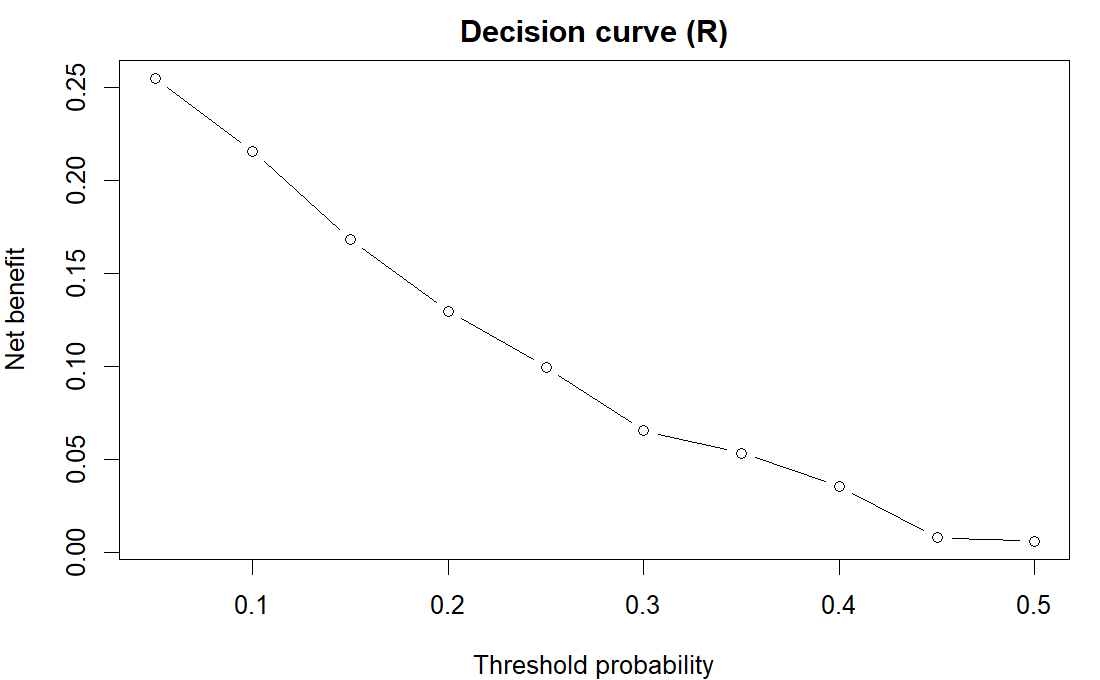
R output. Result:
[1] 0.255 0.216 0.168 0.130 0.100 0.065 0.054 0.036 0.008 0.006# OMOP cohort: net benefit of the model across threshold probabilities. # cohort.csv, one row per person: age = age in years; sex = sex (M/F); comorbidity = comorbidity count; exposed = drug exposure, 0/1; outcome = outcome condition, 0/1. import numpy as np, matplotlib.pyplot as plt import pandas as pd, statsmodels.formula.api as smf coh = pd.read_csv("https://paulinadelmundomd.com/data/omop/cohort.csv") p = smf.logit("outcome ~ age + C(sex) + comorbidity + exposed", coh).fit(disp=0).predict() y = coh.outcome.values; n = len(y); pt = np.arange(.05, .5, .05) nb = [(np.sum((p>t)&(y==1)) - np.sum((p>t)&(y==0))*(t/(1-t)))/n for t in pt] plt.plot(pt, nb, "o-"); plt.xlabel("Threshold probability"); plt.ylabel("Net benefit") plt.title("Decision curve (Python)"); plt.show()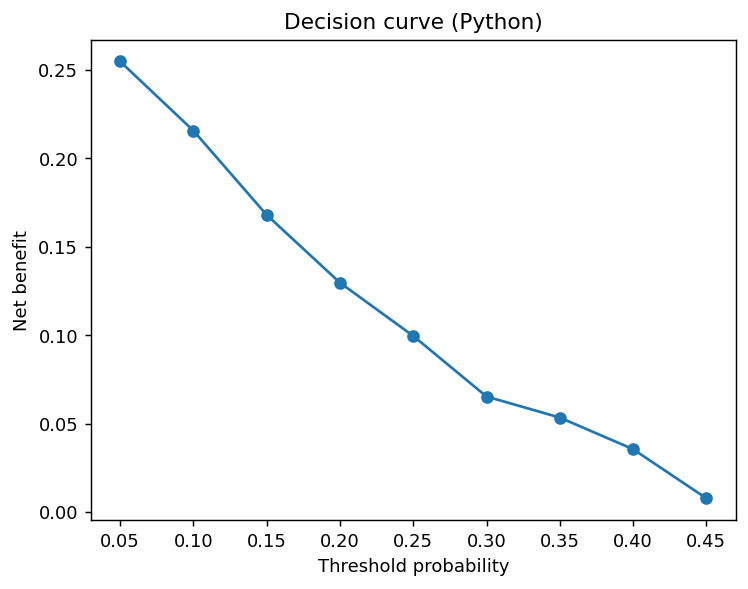
Python output. - Delphi method
- A consensus method where an expert panel answers in iterative anonymous rounds, revising after seeing a statistical summary, so opinion converges without face-to-face pressure. in the pathway →
- Delphi technique
- A structured, iterative way of gathering expert opinion and letting it converge toward consensus, used here to help pin down a study’s objectives and information requirements. in the pathway → · Dohoo, Martin & Stryhn, 2012
- Delta method
-
A way to approximate the variance of a nonlinear function of an estimate from a first-order Taylor expansion, used for example to put a confidence interval on a log odds ratio or a ratio of rates. in the pathway →
\[\operatorname{Var}\!\big(g(\hat\theta)\big) \approx g'(\hat\theta)^{2}\,\operatorname{Var}(\hat\theta)\]
where \(g\) is the transformation and \(g'\) its derivative at \(\hat\theta\).
The odds ratio’s SE (0.13) comes from the coefficient’s SE scaled by the OR itself, a first-order Taylor approximation. It is how software reports an OR’s uncertainty; for skewed transforms the interval is better built on the log scale and exponentiated.
# OMOP cohort: the delta method approximates the SE of a nonlinear transform.
# Here the SE of the odds ratio exp(b) from the SE of the log-odds coefficient
# b: SE(OR) = OR * SE(b). cohort.csv: outcome, exposed, age, comorbidity.
coh <- read.csv("https://paulinadelmundomd.com/data/omop/cohort.csv")
m <- glm(outcome ~ exposed + age + comorbidity, binomial, coh)
b <- coef(m)["exposed"]; se <- sqrt(vcov(m)["exposed", "exposed"])
unname(exp(b) * se)             # delta-method SE of the odds ratio
Result:
[1] 0.1300303# OMOP cohort: the delta method approximates the SE of a nonlinear transform. # Here the SE of the odds ratio exp(b) from the SE of the log-odds coefficient # b: SE(OR) = OR * SE(b). cohort.csv: outcome, exposed, age, comorbidity. import pandas as pd, numpy as np, statsmodels.formula.api as smf coh = pd.read_csv("https://paulinadelmundomd.com/data/omop/cohort.csv") m = smf.logit("outcome ~ exposed + age + comorbidity", coh).fit(disp=0) float(np.exp(m.params["exposed"]) * m.bse["exposed"]) # delta-method SE of the ORResult:
0.13003029140218567 - Deductive reasoning
- Starting from a general hypothesis, working out what must follow, then holding that prediction up against data. In its strong form the goal is not to confirm the hypothesis but to expose it to a test that could break it (see refutationism), which is why a study is framed around a falsifiable prediction rather than a hope. Contrast inductive reasoning. in the pathway → · Rothman & Greenland, 2005
- Density (risk-set) sampling
- Sampling case-control controls from those still at risk at each case’s event time. The payoff: the odds ratio estimates the rate ratio directly, even for a common disease, so no rare-disease assumption is needed. It works because sampling at a constant rate makes the control ratio mirror the person-time ratio, \(b_1/b_0 \approx T_1/T_0\), so \(\dfrac{a_1/b_1}{a_0/b_0}\) estimates \(\dfrac{A_1/T_1}{A_0/T_0}\). It also removes time-window bias. Contrast cumulative sampling. in the pathway → · Dohoo, Martin & Stryhn, 2012
- Descriptive epidemiology
- Describing a health event by person, place, and time to generate hypotheses and fix the frequency measure reported. in the pathway →
- Design effect
-
When you sample in groups (clusters) rather than individuals, people in the same group resemble each other, so each adds less new information and variance inflates. The design effect is how much you must scale up the sample size to make up for it. For clustering it is \(\text{deff}=1+(m-1)\rho\), with \(m\) the cluster size and \(\rho\) the intraclass correlation. in the pathway → · Dohoo, Martin & Stryhn, 2012
\[\text{DEFF} = \frac{\text{Var}_{\text{complex}}}{\text{Var}_{\text{SRS}}}\]
where \(\text{DEFF}\) is the design effect, the variance penalty from the complex design; \(\text{Var}_{\text{complex}}\) is the variance under the actual complex sampling design; \(\text{Var}_{\text{SRS}}\) is the variance a simple random sample of the same size would give.
Clustering inflates the variance by 1.58 times, so the sample carries only about 63% of the information its size suggests. Any analysis that ignores the clusters will report standard errors that are too small.
# Design effect for a cluster of size m with intracluster correlation rho.
m <- 30; rho <- 0.02
1 + (m - 1) * rho   # variance-inflation factor
Result:
[1] 1.58# Design effect for a cluster of size m with intracluster correlation rho. m, rho = 30, 0.02 1 + (m - 1) * rho # variance-inflation factorResult:
1.58 - Detailed balance
- The condition that a move from state A to B is as likely as the reverse move from B to A, which pins a Markov chain’s long-run distribution to the target you want to sample. Metropolis-Hastings enforces it through its accept-reject step. in the pathway → \[p(\theta)\,T(\theta \to \theta') = p(\theta')\,T(\theta' \to \theta)\] where \(T\) is the transition kernel and \(p\) the target distribution.
- Detection bias
- Differential ascertainment of the outcome by exposure group, also called observer bias. in the pathway →
- Deviance
-
A likelihood-based measure of a model’s lack of fit, \(D=-2\ln(\hat{L})\), comparing the fitted model against a saturated one that fits perfectly; smaller is better. Differences in deviance between nested models follow a chi-squared distribution and underlie the likelihood-ratio test, while per-observation deviance residuals feed goodness-of-fit checks and outlier detection in logistic and other GLMs. It generalises the residual sum of squares of a linear model. in the pathway → · Dohoo, Martin & Stryhn, 2012
Residual deviance (1130) measures how far the fit sits from a perfect (saturated) model. Differences in deviance between nested models are the likelihood-ratio test; add 2k or log(n)*k and you get AIC or BIC.
# OMOP cohort: residual deviance of a logistic model, D = -2 ln L, its
# likelihood-based lack of fit and the building block of AIC, BIC, and the
# likelihood-ratio test. cohort.csv: outcome, age, comorbidity.
coh <- read.csv("https://paulinadelmundomd.com/data/omop/cohort.csv")
deviance(glm(outcome ~ age + comorbidity, binomial, coh))   # residual deviance
Result:
[1] 1129.971# OMOP cohort: residual deviance of a logistic model, D = -2 ln L, its # likelihood-based lack of fit and the building block of AIC, BIC, and the # likelihood-ratio test. cohort.csv: outcome, age, comorbidity. import pandas as pd, statsmodels.formula.api as smf, statsmodels.api as sm coh = pd.read_csv("https://paulinadelmundomd.com/data/omop/cohort.csv") float(smf.glm("outcome ~ age + comorbidity", data=coh, family=sm.families.Binomial()).fit().deviance) # residual devianceResult:
1129.9711684596537 - Deviance information criterion (DIC)
- A Bayesian model-comparison criterion, analogous to AIC for MCMC fits: it adds the posterior-mean deviance to an estimate of the effective number of parameters, rewarding fit while penalising complexity, with lower values preferred. It reads straight off an MCMC run but is known to misbehave for mixed models with many random effects, where alternatives such as WAIC are more reliable. in the pathway → · Dohoo, Martin & Stryhn, 2012
- Diagnostic-accuracy studies
- Study design measuring how well an index test discriminates disease against a reference standard, prone to spectrum, verification, and incorporation bias. in the pathway →
- Difference-in-differences
-
A causal design that compares the before-to-after change in a treated group with the change in an untreated group, so anything common to both cancels. It rests on the parallel-trends assumption: absent the treatment, the two groups would have moved in step. in the pathway → · Dimick & Ryan, 2014
\[\text{DiD} = (\bar{Y}^{\text{post}}_T - \bar{Y}^{\text{pre}}_T) - (\bar{Y}^{\text{post}}_C - \bar{Y}^{\text{pre}}_C)\]
where the treated group change from pre to post, minus the control group change; it removes time-invariant confounding under the parallel-trends assumption.
The interaction term, about -4.4 with p=0.017, is the DiD estimate: the treated group’s change over time fell short of the control group’s by 4.4 units. It assumes the two groups would have moved in parallel without treatment.
# CDISC ADaM ADQS: difference-in-differences (2 arms, baseline vs Week 24).
# adqs.csv, one row per subject-visit: AVISIT = visit label; AVAL = score at that visit; TRTP = treatment label.
adqs <- read.csv("https://paulinadelmundomd.com/data/cdisc/adqs.csv")
d <- subset(adqs, AVISIT %in% c("Baseline","Week 24") & TRTP %in% c("Placebo","Xanomeline High Dose"))
d$post <- as.integer(d$AVISIT=="Week 24"); d$active <- as.integer(d$TRTP!="Placebo")
summary(lm(AVAL ~ post * active, data = d))$coefficients   # post:active is the DiD
Result:
              Estimate Std. Error    t value     Pr(>|t|)
(Intercept) 24.0747368  0.8931379 26.9552289 1.457787e-88
post         1.3600000  1.2630877  1.0767265 2.823195e-01
active       0.9082177  1.2879611  0.7051593 4.811646e-01
post:active -4.3634091  1.8214520 -2.3955663 1.710199e-02
# CDISC ADaM ADQS: difference-in-differences (2 arms, baseline vs Week 24). # adqs.csv, one row per subject-visit: AVAL = score at that visit. import pandas as pd, statsmodels.formula.api as smf adqs = pd.read_csv("https://paulinadelmundomd.com/data/cdisc/adqs.csv") d = adqs[adqs.AVISIT.isin(["Baseline","Week 24"]) & adqs.TRTP.isin(["Placebo","Xanomeline High Dose"])].copy() d["post"] = (d.AVISIT=="Week 24").astype(int); d["active"] = (d.TRTP!="Placebo").astype(int) smf.ols("AVAL ~ post * active", d).fit().params # post:active is the DiD estimateResult:
Intercept 24.074737 post 1.360000 active 0.908218 post:active -4.363409 dtype: float64 - Differential misclassification
- Measurement error related to the outcome, which can bias an effect in either direction and is harder to reason about. in the pathway →
- Dimensionality reduction
-
Compressing many correlated variables into a few, through PCA or nonlinear methods. in the pathway →
The first principal component captures 41% of the variance across the six county variables, compressing them onto one axis. PCA trades a little information for far fewer, decorrelated features, useful for visualization or as model inputs.
# ACS counties: principal component analysis on six standardized county
# variables; the first component's share of total variance is how much a single
# combined axis captures. counties.csv, one row per US county.
cty <- read.csv("https://paulinadelmundomd.com/data/acs/counties.csv")
pc <- prcomp(cty[, c("median_income", "poverty_pct", "population",
                     "bachelors_pct", "median_age", "land_sqmi")], scale. = TRUE)
(pc$sdev^2 / sum(pc$sdev^2))[1]   # variance explained by PC1
Result:
[1] 0.4072017# ACS counties: principal component analysis on six standardized county # variables; the first component's share of total variance is how much a single # combined axis captures. counties.csv, one row per US county. import pandas as pd from sklearn.preprocessing import StandardScaler from sklearn.decomposition import PCA cty = pd.read_csv("https://paulinadelmundomd.com/data/acs/counties.csv") cols = ["median_income", "poverty_pct", "population", "bachelors_pct", "median_age", "land_sqmi"] X = StandardScaler().fit_transform(cty[cols]) float(PCA().fit(X).explained_variance_ratio_[0]) # variance explained by PC1Result:
0.40720173608175486 - Direct standardization
-
Removing confounding by a factor such as age when comparing populations by applying each population’s stratum-specific rates to one shared standard structure, \(I_{\text{dir}} = \sum_j w_j I_j\) with standard weights \(w_j\). It yields a fair comparison but applies fixed external weights regardless of how precisely each stratum’s rate is estimated, so a rate resting on few individuals counts for its full standard weight, as much as a stable one. See age-standardization. in the pathway → · Dohoo, Martin & Stryhn, 2012
Standardized to the same age distribution, the exposed rate (0.274) sits below the unexposed (0.311), a contrast the crude comparison could distort if the groups differ in age. Each group’s stratum rates are applied to one shared standard population.
# OMOP cohort: directly standardize the exposed and unexposed outcome rates to a
# common (whole-cohort) age structure, removing age confounding so the two are
# comparable. cohort.csv: age, exposed (0/1), outcome (0/1).
coh <- read.csv("https://paulinadelmundomd.com/data/omop/cohort.csv")
coh$ageg <- cut(coh$age, c(0, 40, 55, 70, Inf)); w <- prop.table(table(coh$ageg))
re <- tapply(coh$outcome[coh$exposed == 1], coh$ageg[coh$exposed == 1], mean)
ru <- tapply(coh$outcome[coh$exposed == 0], coh$ageg[coh$exposed == 0], mean)
unname(c(sum(re * w), sum(ru * w)))   # standardized exposed, unexposed
Result:
[1] 0.2742787 0.3107774# OMOP cohort: directly standardize the exposed and unexposed outcome rates to a # common (whole-cohort) age structure, removing age confounding so the two are # comparable. cohort.csv: age, exposed (0/1), outcome (0/1). import pandas as pd, numpy as np coh = pd.read_csv("https://paulinadelmundomd.com/data/omop/cohort.csv") coh["ageg"] = pd.cut(coh.age, [0, 40, 55, 70, np.inf]); w = coh.ageg.value_counts(normalize=True) re = coh[coh.exposed == 1].groupby("ageg").outcome.mean() ru = coh[coh.exposed == 0].groupby("ageg").outcome.mean() np.array([float((re * w).sum()), float((ru * w).sum())]) # standardized exposed, unexposedResult:
array([0.27427866, 0.3107774 ]) - Discounting
-
Converting future costs and effects to present value over a model’s time horizon. in the pathway →
\[\text{PV} = \sum_t \dfrac{X_t}{(1+r)^t}\]
where \(X_t\) is a cost or benefit in year \(t\) and \(r\) the annual discount rate; future costs and health are worth less in present value, conventionally discounted at about 3 percent.
A $10,000 cost a decade out is worth about $7,441 today at 3%. Cost-effectiveness models discount future costs and future QALYs, usually at the same rate, so a benefit years away is not counted at par with one today.
# Discounting converts a future cost or health effect to present value,
# PV = FV / (1 + r)^t. Here $10,000 arriving in 10 years at a 3% annual rate.
FV <- 10000; r <- 0.03; t <- 10
FV / (1 + r)^t                  # present value
Result:
[1] 7440.939# Discounting converts a future cost or health effect to present value, # PV = FV / (1 + r)^t. Here $10,000 arriving in 10 years at a 3% annual rate. FV, r, t = 10000, 0.03, 10 FV / (1 + r)**t # present valueResult:
7440.93914896725 - Discrimination
-
Whether a model ranks higher-risk patients above lower-risk ones, measured by the AUC (area under the ROC curve, the probability the model scores a random case above a random non-case). in the pathway →
An AUC of 0.67 means the model ranks a random case above a random non-case 67% of the time: modest discrimination (0.5 is a coin flip, 1.0 perfect). Discrimination is only half of performance; a model can rank well yet be miscalibrated.
# OMOP cohort: discrimination, the AUC (area under the ROC curve) of a logistic
# model -- the probability it ranks a random case above a random non-case,
# computed from the ranks of the predicted risks. cohort.csv: outcome, predictors.
coh <- read.csv("https://paulinadelmundomd.com/data/omop/cohort.csv")
p <- predict(glm(outcome ~ age + comorbidity + n_visits, binomial, coh), type = "response")
y <- coh$outcome; n1 <- sum(y == 1); n0 <- sum(y == 0)
(sum(rank(p)[y == 1]) - n1 * (n1 + 1) / 2) / (n1 * n0)   # AUC
Result:
[1] 0.6730347# OMOP cohort: discrimination, the AUC (area under the ROC curve) of a logistic # model -- the probability it ranks a random case above a random non-case. # cohort.csv: outcome, predictors. import pandas as pd, statsmodels.formula.api as smf from sklearn.metrics import roc_auc_score coh = pd.read_csv("https://paulinadelmundomd.com/data/omop/cohort.csv") p = smf.logit("outcome ~ age + comorbidity + n_visits", coh).fit(disp=0).predict() float(roc_auc_score(coh.outcome, p)) # AUCResult:
0.6730346915873384 - Disease registry
- A systematically maintained roster of people with a condition or exposure that supplies a standing population for many designs. in the pathway →
- Disease risk score
- A single score summarizing each patient’s predicted outcome risk from their covariates, used to balance comparison groups. It plays the role the propensity score plays, but built from risk of the outcome rather than probability of treatment. in the pathway →
- Dominance
- In cost-effectiveness, an option is dominated when another both costs less and delivers more, so it is dropped before any incremental cost-effectiveness ratio is computed (strong, or strict, dominance). in the pathway →
- Dose-finding and early-phase designs
- Early studies that find the tolerable dose and the efficacy signal before a confirmatory trial. in the pathway →
- Dose-response relationship
-
A pattern in which the outcome changes steadily with the level or duration of exposure, more exposure giving more (or less) effect, rather than an all-or-nothing jump. A monotonic gradient is one of the Hill criteria and strengthens a causal reading, since confounding rarely mimics a smooth trend, though a threshold or plateau shape is also biologically common. It is best examined by modelling exposure continuously, with splines or fractional polynomials, rather than dichotomising, which can hide or manufacture a gradient. in the pathway → · Dohoo, Martin & Stryhn, 2012
Each additional comorbidity multiplies the odds of the outcome by about 1.08. A consistent gradient is one of the Bradford Hill viewpoints, strengthening but never proving a causal reading.
# OMOP cohort: a dose-response reading, the odds ratio per additional
# comorbidity, from a logistic model treating comorbidity count as a graded
# exposure. A steady OR above 1 is a monotonic gradient. cohort.csv.
coh <- read.csv("https://paulinadelmundomd.com/data/omop/cohort.csv")
unname(exp(coef(glm(outcome ~ comorbidity, binomial, coh))["comorbidity"]))   # OR per comorbidity
Result:
[1] 1.076459# OMOP cohort: a dose-response reading, the odds ratio per additional # comorbidity, from a logistic model treating comorbidity count as a graded # exposure. A steady OR above 1 is a monotonic gradient. cohort.csv. import pandas as pd, numpy as np, statsmodels.formula.api as smf coh = pd.read_csv("https://paulinadelmundomd.com/data/omop/cohort.csv") float(np.exp(smf.logit("outcome ~ comorbidity", coh).fit(disp=0).params["comorbidity"]))Result:
1.076458979093734 - Double-barreled question
- A survey item that asks two things at once. in the pathway →
- Double-barrelled question
- A single question that quietly asks two things at once (for instance whether a disease is serious and whether people should be vaccinated), so no one answer is interpretable; the fix is to split it into two questions. in the pathway → · Dohoo, Martin & Stryhn, 2012
- Double-programming
- Independent re-derivation of a dataset or output by a second programmer without seeing the first, reconciled value by value as the sign-off. in the pathway →
- Doubly robust
-
A property of estimators that fit two models, one for treatment and one for the outcome, and land on the right answer if at least one of the two is correct. You get two chances instead of one: the bias is proportional to the product of the two models’ errors, so a small error in either keeps the bias small. The name oversells it, though. It offers no protection against unmeasured confounding, none when both models are wrong (the error product no longer vanishes), and none when positivity fails and a near-zero propensity score makes the correction term explode even under a perfect outcome model. Doubly robust is insurance, not a guarantee. in the pathway → · Tsiatis, 2006
The adjusted effect is about -0.046 on the risk scale, roughly 4.6 fewer events per 100. It is consistent if either the outcome model or the treatment model is correctly specified, and you do not need both.
# OMOP cohort: doubly-robust (AIPW) risk difference, PS + outcome models.
# cohort.csv, one row per person: age = age in years; sex = sex (M/F); comorbidity = comorbidity count; exposed = drug exposure, 0/1; outcome = outcome condition, 0/1.
coh <- read.csv("https://paulinadelmundomd.com/data/omop/cohort.csv")
ps <- predict(glm(exposed ~ age + sex + comorbidity, data = coh, family = binomial), type="response")
om <- glm(outcome ~ exposed + age + sex + comorbidity, data = coh, family = binomial)
m1 <- predict(om, transform(coh, exposed=1), type="response")
m0 <- predict(om, transform(coh, exposed=0), type="response")
A <- coh$exposed; Y <- coh$outcome
mean(m1 + A*(Y-m1)/ps) - mean(m0 + (1-A)*(Y-m0)/(1-ps))   # AIPW risk difference
Result:
[1] -0.04576048# OMOP cohort: doubly-robust (AIPW) risk difference, PS + outcome models. # cohort.csv, one row per person: age = age in years; sex = sex (M/F); comorbidity = comorbidity count; exposed = drug exposure, 0/1; outcome = outcome condition, 0/1. import numpy as np, pandas as pd, statsmodels.formula.api as smf coh = pd.read_csv("https://paulinadelmundomd.com/data/omop/cohort.csv") ps = smf.logit("exposed ~ age + C(sex) + comorbidity", coh).fit(disp=0).predict() om = smf.logit("outcome ~ exposed + age + C(sex) + comorbidity", coh).fit(disp=0) m1 = om.predict(coh.assign(exposed=1)); m0 = om.predict(coh.assign(exposed=0)) A, Y = coh.exposed, coh.outcome np.mean(m1 + A*(Y-m1)/ps) - np.mean(m0 + (1-A)*(Y-m0)/(1-ps)) # AIPW risk differenceResult:
-0.045760480970088224 - Doubly-robust estimators
- Estimators such as augmented IPW and TMLE that combine a propensity and an outcome model and stay consistent if either is right. in the pathway → \[\hat\mu_1 = \underbrace{\dfrac{1}{n}\sum_i \dfrac{A_i Y_i}{\hat e_i}}_{\text{IPW}} \;-\; \underbrace{\dfrac{1}{n}\sum_i \dfrac{A_i-\hat e_i}{\hat e_i}\,\hat m_1(X_i)}_{\text{augmentation}}\] where \(\hat e\) is the propensity and \(\hat m_1\) the outcome model. The first term is the inverse-probability-weighted mean; the second augments it using \(\hat m_1\). If \(\hat e\) is correct the augmentation has mean zero, and if \(\hat m_1\) is correct the weighting errors cancel, so \(\hat\mu_1\) stays consistent when either model is right (augmented IPW).
- Drug era (OMOP)
- A derived continuous exposure span in the OMOP model built from raw drug records using an explicit persistence gap. in the pathway →
- Dummy variable
-
An indicator coding of a categorical predictor: a \(k\)-level factor becomes \(k-1\) binary variables, each contrasting one level against a held-out reference category, so the model estimates every level’s shift from that baseline. Omitting one level avoids perfect collinearity with the intercept; the choice of reference changes how the coefficients read but not the fit. Ordered factors can instead take hierarchical or polynomial coding when the spacing between levels matters. in the pathway → · Dohoo, Martin & Stryhn, 2012
The three ORs (1.30, 1.73, 1.75) give each age band’s odds relative to the youngest. A k-level factor needs k-1 dummies, not k: including all k plus an intercept makes the design collinear, the dummy-variable trap.
# OMOP cohort: a four-level age factor becomes three 0/1 dummy variables, each
# contrasting its level with the reference (the youngest group). The logistic
# ORs are each level's effect relative to that reference. cohort.csv: age, outcome.
coh <- read.csv("https://paulinadelmundomd.com/data/omop/cohort.csv")
coh$ageg <- cut(coh$age, c(0, 40, 55, 70, Inf))
unname(exp(coef(glm(outcome ~ ageg, binomial, coh)))[-1])   # OR for each non-reference level
Result:
[1] 1.299642 1.730901 1.745283# OMOP cohort: a four-level age factor becomes three 0/1 dummy variables, each # contrasting its level with the reference (the youngest group). The logistic # ORs are each level's effect relative to that reference. cohort.csv: age, outcome. import pandas as pd, numpy as np, statsmodels.formula.api as smf coh = pd.read_csv("https://paulinadelmundomd.com/data/omop/cohort.csv") coh["ageg"] = pd.cut(coh.age, [0, 40, 55, 70, np.inf]) np.exp(smf.logit("outcome ~ C(ageg)", coh).fit(disp=0).params.values[1:]) # OR per levelResult:
array([1.29964158, 1.73090129, 1.74528302]) - Dynamic transmission model
- An infectious-disease model capturing how treating one person changes others’ risk through herd immunity, which a fixed-risk cohort model cannot. in the pathway →
E
- Early stopping
- Halting an iterative learner such as boosting, gradient descent, or a neural network once held-out error stops improving, so the extra iterations that would start fitting noise are never taken. It regularizes through training time rather than an explicit penalty. in the pathway →
- Ecological study
-
A study whose unit of analysis is a group (countries, regions, time periods) rather than an individual, correlating a group’s average exposure with its average outcome, as in a plot of national fat intake against heart-disease rates. It is cheap and handy for generating hypotheses and for studying group-level exposures like policies or air quality, but associations between group averages need not hold within individuals, the ecological fallacy. Multilevel models that keep both individual and group data avoid that trap. in the pathway → · Dohoo, Martin & Stryhn, 2012
The strong county-level correlation (-0.79) is a property of counties, not people. Reading it as an individual-level relationship is the ecological fallacy: the aggregate association can differ in size, or even sign, from the one within individuals.
# ACS counties: an ecological (group-level) correlation -- the unit is the
# county, not the person. Higher-poverty counties have lower median income.
# counties.csv, one row per US county.
cty <- read.csv("https://paulinadelmundomd.com/data/acs/counties.csv")
cor(cty$poverty_pct, cty$median_income)   # county-level correlation
Result:
[1] -0.7899105# ACS counties: an ecological (group-level) correlation -- the unit is the # county, not the person. Higher-poverty counties have lower median income. # counties.csv, one row per US county. import pandas as pd cty = pd.read_csv("https://paulinadelmundomd.com/data/acs/counties.csv") float(cty.poverty_pct.corr(cty.median_income)) # county-level correlationResult:
-0.7899105371292241 - Effect modification
-
When an exposure’s effect differs across levels of a third variable, a real feature to estimate and report by subgroup, distinct from confounding; on a model it appears as an interaction. in the pathway →
Exposure looks protective among the younger (OR 0.75) but nearly null among the older (0.96): the effect is modified by age. Unlike confounding, effect modification is estimated and reported rather than adjusted away, because the answer genuinely depends on the modifier.
# OMOP cohort: the exposure odds ratio within younger and older strata (split at
# the median age). Differing ORs across strata are effect modification, a real
# feature to report, not a bias to remove. cohort.csv: outcome, exposed, age.
coh <- read.csv("https://paulinadelmundomd.com/data/omop/cohort.csv")
coh$old <- coh$age >= median(coh$age)
unname(c(exp(coef(glm(outcome ~ exposed, binomial, coh[!coh$old, ]))["exposed"]),
         exp(coef(glm(outcome ~ exposed, binomial, coh[coh$old, ]))["exposed"])))
Result:
[1] 0.7548387 0.9629630# OMOP cohort: the exposure odds ratio within younger and older strata (split at # the median age). Differing ORs across strata are effect modification, a real # feature to report, not a bias to remove. cohort.csv: outcome, exposed, age. import pandas as pd, numpy as np, statsmodels.formula.api as smf coh = pd.read_csv("https://paulinadelmundomd.com/data/omop/cohort.csv") coh["old"] = coh.age >= coh.age.median() oy = np.exp(smf.logit("outcome ~ exposed", coh[~coh.old]).fit(disp=0).params["exposed"]) oo = np.exp(smf.logit("outcome ~ exposed", coh[coh.old]).fit(disp=0).params["exposed"]) np.array([float(oy), float(oo)]) # OR in younger, olderResult:
array([0.75483871, 0.96296296]) - Effect size
- The magnitude of a difference or association, given in raw units or standardized as Cohen’s d, an odds ratio, or a hazard ratio. It is the numerator of a power calculation, so the smaller the effect worth detecting, the larger the sample required. in the pathway →
- Efficiency frontier
- The options left after removing the dominated and extended-dominated ones, ordered by effect; the incremental cost-effectiveness ratios are the slopes between adjacent options along it. in the pathway →
- Epidemic curve
- A histogram of case counts by time of onset, the first picture drawn in any outbreak investigation. Its shape is diagnostic: a sharp single peak suggests a point-source exposure, successive peaks spaced by the serial interval suggest person-to-person spread, and a sustained plateau suggests a continuing common source. The rising limb also gives a quick read on the growth rate and hence \(R_0\). in the pathway → · Dohoo, Martin & Stryhn, 2012
- E-value
-
A measure of how strong a hidden confounder would have to be, in association with both treatment and outcome, to explain away an observed result. in the pathway → · VanderWeele & Ding, 2017
\[E = \text{RR} + \sqrt{\text{RR}(\text{RR} - 1)}\]
where \(E\) is the E-value, the smallest association a hidden confounder would need with both treatment and outcome to explain the estimate away; \(\text{RR}\) is the observed risk ratio, taken above 1 (for a protective effect, apply the formula to its reciprocal).
An unmeasured confounder would need to be associated with both exposure and outcome by a risk ratio of about 3, beyond the measured covariates, to explain the finding away. Larger E-values mean the result is more robust to confounding.
# E-value from an observed risk ratio (VanderWeele-Ding).
RR <- 1.8
RR + sqrt(RR * (RR - 1))   # confounding strength needed to explain it away
Result:
[1] 3# E-value from an observed risk ratio (VanderWeele-Ding). RR = 1.8 RR + (RR * (RR - 1))**0.5 # confounding strength needed to explain it awayResult:
3.0 - Ecological fallacy
- Reading a group-level association as if it held for individuals, a trap of aggregated data. in the pathway →
- Effect measures
-
The scales for reporting a result, including relative measures like risk, rate, and odds ratios and absolute measures like risk difference and number needed to treat. in the pathway → · Dohoo, Martin & Stryhn, 2012
\[\text{RR} = \frac{\text{risk}_{\text{exposed}}}{\text{risk}_{\text{unexposed}}}, \quad \text{RD} = \text{risk}_{\text{exposed}} - \text{risk}_{\text{unexposed}}\]
where \(\text{RR}\) is the risk ratio, a relative measure; \(\text{RD}\) is the risk difference, an absolute measure; \(\text{risk}_{\text{exposed}}\) is the outcome risk in the exposed group; \(\text{risk}_{\text{unexposed}}\) is the outcome risk in the unexposed group.
For the same data the risk ratio is 0.84, the odds ratio 0.79, and the risk difference -0.05. Relative measures travel better across populations; the absolute risk difference is what a patient feels and what the number needed to treat inverts.
# OMOP cohort: three effect measures for the same exposure-outcome table -- the
# risk ratio and odds ratio (relative) and the risk difference (absolute).
# cohort.csv: exposed (0/1), outcome (0/1).
coh <- read.csv("https://paulinadelmundomd.com/data/omop/cohort.csv")
r1 <- mean(coh$outcome[coh$exposed == 1]); r0 <- mean(coh$outcome[coh$exposed == 0])
c(r1/r0, (r1/(1-r1)) / (r0/(1-r0)), r1 - r0)   # RR, OR, RD
Result:
[1] 0.8447156 0.7880178 -0.0491682# OMOP cohort: three effect measures for the same exposure-outcome table -- the # risk ratio and odds ratio (relative) and the risk difference (absolute). # cohort.csv: exposed (0/1), outcome (0/1). import pandas as pd, numpy as np coh = pd.read_csv("https://paulinadelmundomd.com/data/omop/cohort.csv") r1 = coh.outcome[coh.exposed == 1].mean(); r0 = coh.outcome[coh.exposed == 0].mean() np.array([r1/r0, (r1/(1-r1)) / (r0/(1-r0)), r1 - r0]) # RR, OR, RDResult:
array([ 0.84471563, 0.7880178 , -0.0491682 ]) - Effective sample size
-
The sample size discounted by the design effect, \(\text{ESS} = \left(\sum_i w_i\right)^2 / \sum_i w_i^2\), so a design effect of 2 leaves the precision of half the respondents. The same quantity gauges how much information inverse-probability weights retain: a value far below the sample size flags a few extreme weights dominating the estimate. in the pathway → · Kish, 1965
\[n_{\text{eff}} = \frac{n}{\text{DEFF}}\]
where \(n_{\text{eff}}\) is the effective sample size, the precision the design actually delivers; \(n\) is the achieved sample size; \(\text{DEFF}\) is the design effect, the variance penalty from clustering and unequal weighting.
After the design effect, 1000 clustered observations carry the information of about 633 independent ones. Power and CI width should be judged against this smaller number, not the raw count.
# Effective sample size after clustering: n / design effect.
n <- 1000; deff <- 1 + (30 - 1) * 0.02
n / deff
Result:
[1] 632.9114# Effective sample size after clustering: n / design effect. n, deff = 1000, 1 + (30 - 1) * 0.02 n / deffResult:
632.9113924050632 - Egger’s test
-
A statistical test for funnel-plot asymmetry, used to check for publication bias. in the pathway →
Both languages run the same Egger (1997) regression, so they agree: the intercept is about -2.37 with p=0.35, giving no evidence of funnel-plot asymmetry. It is the intercept, not the slope on precision, that is the asymmetry test; a nonzero intercept would signal small-study or publication bias. With only 12 studies the test is low-powered, so a null does not prove symmetry. (R’s metafor::regtest reports a related but not identical number, because its default weights the regression by the studies’ variances and heterogeneity and tests it with a z rather than a t.)
# Egger's test (1997): regress the standard normal deviate on precision;
# a nonzero INTERCEPT flags funnel-plot asymmetry (small-study / publication bias).
# studies.csv, one row per trial: yi = effect estimate (log OR); sei = standard error of yi.
d <- read.csv("https://paulinadelmundomd.com/data/meta/studies.csv")
snd <- d$yi / d$sei; precision <- 1 / d$sei          # standard normal deviate, precision
coef(summary(lm(snd ~ precision)))["(Intercept)", ]  # intercept = the asymmetry test
Result:
  Estimate Std. Error    t value   Pr(>|t|)
-2.3662353  2.4110661 -0.9814062  0.3495395
# Egger's test (1997): regress the standard normal deviate on precision; # a nonzero INTERCEPT flags funnel-plot asymmetry (small-study / publication bias). # studies.csv, one row per trial: yi = effect estimate (log OR); sei = standard error of yi. import numpy as np, pandas as pd, statsmodels.api as sm d = pd.read_csv("https://paulinadelmundomd.com/data/meta/studies.csv") snd = d.yi.values / d.sei.values; precision = 1 / d.sei.values # standard normal deviate, precision m = sm.OLS(snd, sm.add_constant(precision)).fit() m.params[0], m.bse[0], m.tvalues[0], m.pvalues[0] # intercept, SE, t, p = the asymmetry testResult:
(np.float64(-2.3662352564415063), np.float64(2.411066123780885), np.float64(-0.9814062057870575), np.float64(0.3495394672897948)) - Elastic net
-
A regularization that blends ridge and lasso penalties. in the pathway →
\[\hat\beta = \operatorname*{arg\,min}_{\beta}\ \lVert Y - X\beta\rVert^{2} + \lambda\big[\,\alpha\textstyle\sum_j\lvert\beta_j\rvert + (1-\alpha)\textstyle\sum_j\beta_j^{2}\,\big]\]
where the squared-error loss is penalized by a blend of the lasso (\(\ell_1\), which zeros coefficients) and ridge (\(\ell_2\), which shrinks them); \(\alpha\) sets the mix and \(\lambda\) the strength. To make R and Python solve the identical problem, predictors are standardized and a single \(\lambda\) is fixed (rather than cross-validated), with glmnet’s \(\lambda\) mapped to scikit-learn’s \(C = 1/(n\lambda)\).
With predictors standardized and a single lambda fixed, glmnet and scikit-learn now solve the same penalized problem and return the same coefficients. On the standardized scale comorbidity carries the largest weight (about +0.60), age and n_visits keep smaller negative ones, and the L1 part of the penalty has zeroed out sex and exposed. Coefficients are on the log-odds scale and are biased toward zero by design, so read them for direction and relative size rather than as unbiased effects. In practice you would cross-validate lambda instead of fixing it; it is fixed here only so the two languages line up.
# OMOP cohort: elastic-net (alpha = 0.5) logistic regression, standardized, fixed lambda.
# cohort.csv, one row per person: age; sex (M/F); comorbidity; exposed 0/1; n_visits; outcome 0/1.
library(glmnet)
coh <- read.csv("https://paulinadelmundomd.com/data/omop/cohort.csv")
X <- scale(model.matrix(outcome ~ age + sex + comorbidity + exposed + n_visits, coh)[, -1])
fit <- glmnet(X, coh$outcome, family = "binomial", alpha = 0.5, lambda = 0.02, standardize = FALSE)
round(setNames(as.vector(coef(fit)), rownames(coef(fit))), 3)   # named: intercept + 5 coefficients
Result:
(Intercept)         age        sexM comorbidity     exposed    n_visits
     -0.930      -0.162       0.000       0.598       0.000      -0.052
# OMOP cohort: elastic-net (l1_ratio = 0.5) logistic regression, standardized, fixed lambda. # cohort.csv, one row per person: age; sex (M/F); comorbidity; exposed 0/1; n_visits; outcome 0/1. import pandas as pd, numpy as np from sklearn.linear_model import LogisticRegression coh = pd.read_csv("https://paulinadelmundomd.com/data/omop/cohort.csv") X = pd.get_dummies(coh[["age", "sex", "comorbidity", "exposed", "n_visits"]], drop_first=True).astype(float) X = X[["age", "sex_M", "comorbidity", "exposed", "n_visits"]] # match R's column order Xs = (X - X.mean()) / X.std() # standardize like R's scale() lam = 0.02; C = 1 / (len(coh) * lam) # glmnet lambda -> sklearn C fit = LogisticRegression(penalty="elasticnet", l1_ratio=0.5, C=C, solver="saga", max_iter=500000, tol=1e-9).fit(Xs, coh.outcome) dict(zip(["(Intercept)"] + list(X.columns), np.round(np.r_[fit.intercept_, fit.coef_[0]], 3)))Result:
{'(Intercept)': np.float64(-0.93), 'age': np.float64(-0.162), 'sex_M': np.float64(0.0), 'comorbidity': np.float64(0.598), 'exposed': np.float64(0.0), 'n_visits': np.float64(-0.052)} - Electronic health record data
- Clinically rich data recorded for care, so messy, single-system, and informatively missing rather than research-ready. in the pathway →
- Elixhauser comorbidity measures
- A broader set of comorbidity categories, often kept as separate indicators rather than one number, to adjust for diverse baseline conditions. in the pathway → · Elixhauser et al., 1998
- Empirical calibration
- Run many analyses that should show no effect (negative controls), observe how far their estimates scatter from zero, and use that scatter to recalibrate p-values and intervals so they reflect the study’s systematic error, not just sampling error. in the pathway →
- Endpoint adjudication and chart review
- Clinician review of source records, blinded to exposure, serving as the reference standard for validation. in the pathway →
- Endpoint logic and pre-registration
- Fixing the primary endpoint the sample size rests on and publicly committing to it before unblinding, keeping confirmatory analyses confirmatory. in the pathway →
- EQ-5D
- The EuroQol five-dimension questionnaire, a preference-based instrument used to derive the utility weights that anchor quality-adjusted life years. in the pathway → · EuroQol EQ-5D-5L ↗
- Equivalence trial
- A trial that bounds the difference between treatments on both sides. in the pathway →
- Estimand
- The exact quantity to be estimated, pinned down before analysis: which effect, measured how, in whom, and how dropout or other intercurrent events are handled. Fixing it keeps the question from quietly shifting as the analysis proceeds. in the pathway →
- Eta-squared
-
An ANOVA effect-size measure, the share of variance the groups explain. in the pathway →
\[\eta^{2} = \dfrac{\mathrm{SS}_{\text{between}}}{\mathrm{SS}_{\text{total}}}\]
where \(\mathrm{SS}_{\text{between}}\) is the between-group and \(\mathrm{SS}_{\text{total}}\) the total sum of squares.
Outcome group explains under 1% of the variance in age (eta-squared = 0.008), a tiny effect even though the mean-age difference was statistically detectable. Eta-squared is the ANOVA counterpart of R-squared and grows only with real explained variance, not sample size.
# OMOP cohort: eta-squared, the ANOVA effect size -- the share of total variance
# in age explained by outcome group (between-group SS / total SS).
# cohort.csv: age, outcome.
coh <- read.csv("https://paulinadelmundomd.com/data/omop/cohort.csv")
grand <- mean(coh$age); SSt <- sum((coh$age - grand)^2)
SSb <- sum(tapply(coh$age, coh$outcome, function(x) length(x) * (mean(x) - grand)^2))
SSb / SSt                       # eta-squared
Result:
[1] 0.007864248# OMOP cohort: eta-squared, the ANOVA effect size -- the share of total variance # in age explained by outcome group (between-group SS / total SS). # cohort.csv: age, outcome. import pandas as pd coh = pd.read_csv("https://paulinadelmundomd.com/data/omop/cohort.csv") grand = coh.age.mean(); SSt = ((coh.age - grand) ** 2).sum() SSb = coh.groupby("outcome").age.apply(lambda x: len(x) * (x.mean() - grand) ** 2).sum() float(SSb / SSt) # eta-squaredResult:
0.00786424797442241 - Evidence-to-decision
- Frameworks making the move from evidence to a recommendation explicit, weighing benefits and harms alongside values, feasibility, equity, and cost. in the pathway →
- EVPI
- Expected value of perfect information: an upper bound on what further research could be worth, equal to the expected loss from deciding under current uncertainty. in the pathway → \[\text{EVPI} = E_{\theta}\!\big[\max_d U(d,\theta)\big] - \max_d E_{\theta}\!\big[U(d,\theta)\big]\] where the expected payoff if all parameter uncertainty \(\theta\) were resolved before deciding, minus the payoff under current uncertainty; a large EVPI relative to study cost argues for more research.
- Exact confidence interval
-
A confidence interval built from the exact sampling distribution instead of a normal approximation: the binomial (Clopper-Pearson) interval for a proportion, or a Poisson-based interval for a rate. It is preferred when counts are small or the frequency is near 0 or 1, where the approximate \(\hat\theta \pm Z\,\text{SE}\) interval can mislead or fall outside \([0,1]\). in the pathway → · Dohoo, Martin & Stryhn, 2012
The exact interval [0.264, 0.321] closely tracks the normal-approximation one here because n is large and the rate is mid-range. The exact method earns its keep when counts are small or the proportion is near 0 or 1, where the normal approximation can stray outside [0, 1].
# OMOP cohort: an exact (Clopper-Pearson) 95% confidence interval for the outcome
# proportion, built from the binomial distribution rather than a normal
# approximation, so it stays valid for small samples or extreme rates.
# cohort.csv: outcome (0/1).
coh <- read.csv("https://paulinadelmundomd.com/data/omop/cohort.csv")
as.numeric(binom.test(sum(coh$outcome), nrow(coh))$conf.int)   # exact 95% CI
Result:
[1] 0.2639659 0.3212644# OMOP cohort: an exact (Clopper-Pearson) 95% confidence interval for the outcome # proportion, built from the binomial distribution rather than a normal # approximation, so it stays valid for small samples or extreme rates. # cohort.csv: outcome (0/1). import pandas as pd, numpy as np from scipy import stats coh = pd.read_csv("https://paulinadelmundomd.com/data/omop/cohort.csv") ci = stats.binomtest(int(coh.outcome.sum()), len(coh)).proportion_ci(method="exact") np.array([ci.low, ci.high]) # exact 95% CIResult:
array([0.26396589, 0.32126443]) - Exact logistic regression
- Conditions on sufficient statistics and enumerates the permutation distribution, giving valid inference without asymptotic approximations when data are very sparse. in the pathway →
- Etiologic fraction
-
The share of cases among the exposed whose disease their exposure genuinely helped cause, in the sense that it was a component of the sufficient cause that produced them. It is not the same as the attributable (or excess) fraction \((\text{RR}-1)/\text{RR}\), which counts only the excess cases observed: an exposure that merely hastens a disease everyone would get anyway leaves the two risks equal, so the excess fraction is 0 while the etiologic fraction is 1. Because we never learn which sufficient cause produced a given case, the etiologic fraction cannot be estimated from epidemiological data, and the attributable fraction serves only as a lower bound on it. in the pathway → · Rothman, Greenland & Lash, 2008
With a risk ratio of 1.26, about 21% of the outcomes among the older group are attributable to being older, in the sense that they would not have occurred at the younger group’s baseline risk. The fraction assumes the RR is causal, not merely associational.
# OMOP cohort: the attributable (excess) fraction among the exposed,
# AFe = (RR - 1) / RR -- the excess share of exposed cases, a lower bound on the
# (unestimable) etiologic fraction. Exposure: older than median age. cohort.csv.
coh <- read.csv("https://paulinadelmundomd.com/data/omop/cohort.csv")
coh$old <- coh$age >= median(coh$age)
RR <- mean(coh$outcome[coh$old]) / mean(coh$outcome[!coh$old])
(RR - 1) / RR                   # attributable fraction among the exposed
Result:
[1] 0.2069237# OMOP cohort: the attributable (excess) fraction among the exposed, # AFe = (RR - 1) / RR -- the excess share of exposed cases, a lower bound on the # (unestimable) etiologic fraction. Exposure: older than median age. cohort.csv. import pandas as pd coh = pd.read_csv("https://paulinadelmundomd.com/data/omop/cohort.csv") coh["old"] = coh.age >= coh.age.median() RR = coh.outcome[coh.old].mean() / coh.outcome[~coh.old].mean() float((RR - 1) / RR) # attributable fraction among the exposedResult:
0.20692368214004733 - Exchangeability
- The identifiability condition that treated and untreated are comparable once confounders are controlled, meaning no unmeasured confounding; written \(\{Y(0),Y(1)\}\perp T\mid X\), it is also called conditional ignorability. in the pathway → · Dohoo, Martin & Stryhn, 2012
- Exclusion restriction
- The assumption that an instrument affects the outcome only through the exposure, with no direct path of its own. It cannot be tested and must be argued on subject-matter grounds; any other route from the instrument to the outcome biases the instrumental-variable estimate. in the pathway →
- Expectation-maximization
- An iterative maximum-likelihood algorithm for hidden or missing data, alternating an expectation step that fills in the unknowns with a maximization step that updates the parameters. in the pathway →
- Expected value of partial perfect information (EVPPI)
- Prices resolving specific uncertain parameters, identifying which uncertainty is worth further research. in the pathway →
- Expected value of sample information
- A measure valuing a study of a given design and size, going beyond perfect information to price real research. in the pathway →
- Expert determination
- A HIPAA de-identification route where a statistician certifies the re-identification risk is very small. in the pathway →
- Exploratory data analysis (EDA)
- The open-ended first look at data, using summaries and especially plots (histograms, scatterplots, box plots) to learn its shape, spot errors and outliers, check distributions, and see which relationships are worth modelling, before any formal test. Championed by Tukey, it is about generating questions rather than confirming answers, so what it turns up should be treated as hypotheses to test on other data, not conclusions, lest you mistake noise for signal. in the pathway → · Dohoo, Martin & Stryhn, 2012
- Exposure definition in RWD
- Turning prescription or claim records into an exposure variable with a defined start, window, and end so it is clear who is treated and when. in the pathway →
- Exposure episode construction
- Building a continuous treatment span from individual pharmacy fills: each fill covers its days supplied, consecutive fills are stitched into one episode as long as any gap between running out and the next fill stays within a permissible gap (the grace period), and the episode ends once a gap exceeds it; early refills are either carried forward as stockpile or capped. Because the grace period and the stockpiling rule decide who counts as continuously treated, they are pre-specified, not tuned to the result. in the pathway →
- Extended dominance
- An option is extendedly dominated when its incremental cost-effectiveness ratio is higher than that of a more effective option, so a blend of two other options buys more health per dollar; it is dropped from the efficiency frontier before the final ratios are read. in the pathway →
- External validity
- Whether a study’s result carries beyond the source population to the broader target population it is meant to inform, judged by how representative the source is of the target. It is the study-design face of generalizability, usually easier to defend for an association than for a descriptive figure like a prevalence. in the pathway → · Dohoo, Martin & Stryhn, 2012
- Extract-transform-load
- Pulling from source tables, deriving study variables from operational definitions, and assembling one analysis-ready table. in the pathway →
F
- F1 score
-
The harmonic mean of precision and recall, high only when both are. in the pathway →
\[F_1 = \frac{2 \cdot \text{precision} \cdot \text{recall}}{\text{precision} + \text{recall}}\]
where the harmonic mean is dragged down by whichever of precision and recall is smaller, so the score is high only when both precision and recall are high.
At a prevalence threshold the model’s F1 is 0.49, balancing precision (correct among predicted positives) with recall (caught among true positives). F1 penalizes ignoring either, unlike accuracy, which a model can inflate by predicting the majority class.
# OMOP cohort: F1, the harmonic mean of precision and recall, from a logistic
# classifier thresholded at the outcome prevalence. cohort.csv: outcome, predictors.
coh <- read.csv("https://paulinadelmundomd.com/data/omop/cohort.csv")
p <- predict(glm(outcome ~ age + comorbidity + n_visits, binomial, coh), type = "response")
pred <- as.integer(p >= mean(coh$outcome)); y <- coh$outcome
tp <- sum(pred == 1 & y == 1); fp <- sum(pred == 1 & y == 0); fn <- sum(pred == 0 & y == 1)
prec <- tp / (tp + fp); rec <- tp / (tp + fn)
2 * prec * rec / (prec + rec)   # F1 score
Result:
[1] 0.4857955# OMOP cohort: F1, the harmonic mean of precision and recall, from a logistic # classifier thresholded at the outcome prevalence. cohort.csv: outcome, predictors. import pandas as pd, numpy as np, statsmodels.formula.api as smf coh = pd.read_csv("https://paulinadelmundomd.com/data/omop/cohort.csv") p = np.asarray(smf.logit("outcome ~ age + comorbidity + n_visits", coh).fit(disp=0).predict()) pred = (p >= coh.outcome.mean()).astype(int); y = coh.outcome.to_numpy() tp = ((pred == 1) & (y == 1)).sum(); fp = ((pred == 1) & (y == 0)).sum(); fn = ((pred == 0) & (y == 1)).sum() prec = tp / (tp + fp); rec = tp / (tp + fn) float(2 * prec * rec / (prec + rec)) # F1 scoreResult:
0.48579545454545453 - Factorial design
- A trial that assigns two or more interventions in all combinations at once (a \(2\times2\) design gives neither, each alone, and both), so one study answers several questions and can test their interaction. Because balanced assignment keeps the interventions orthogonal, their main effects are unconfounded and estimated almost as efficiently as in separate trials. It is best kept to two or three factors, beyond which the interactions grow hard to interpret. in the pathway → · Dohoo, Martin & Stryhn, 2012
- Factorial trial
- A trial that tests two or more interventions at once by crossing them in the same subjects, efficient when the interventions do not interact. in the pathway →
- False-discovery rate
- The expected share of false positives among rejections, controlled by Benjamini-Hochberg, better for screening. in the pathway → · Benjamini & Hochberg, 1995 \[\text{FDR} = E\!\left[\dfrac{V}{R}\right]\] where \(V\) is the number of false rejections and \(R\) the total rejections; controlling the FDR (Benjamini-Hochberg) tolerates a known fraction of false positives for more power than family-wise control.
- False positive (FP)
-
A case the model calls positive that is truly negative, a false alarm; it lowers precision and, against the true negatives, specificity. in the pathway →
About 34% of the truly negative patients are flagged positive at this threshold. Each false positive lowers precision, and raising the threshold to cut them trades away recall: the tradeoff a ROC curve traces out.
# OMOP cohort: the false-positive rate (1 - specificity), the share of true
# negatives the classifier wrongly flags positive. cohort.csv: outcome, predictors.
coh <- read.csv("https://paulinadelmundomd.com/data/omop/cohort.csv")
p <- predict(glm(outcome ~ age + comorbidity + n_visits, binomial, coh), type = "response")
pred <- as.integer(p >= mean(coh$outcome)); y <- coh$outcome
sum(pred == 1 & y == 0) / sum(y == 0)   # false-positive rate
Result:
[1] 0.3403955# OMOP cohort: the false-positive rate (1 - specificity), the share of true # negatives the classifier wrongly flags positive. cohort.csv: outcome, predictors. import pandas as pd, numpy as np, statsmodels.formula.api as smf coh = pd.read_csv("https://paulinadelmundomd.com/data/omop/cohort.csv") p = np.asarray(smf.logit("outcome ~ age + comorbidity + n_visits", coh).fit(disp=0).predict()) pred = (p >= coh.outcome.mean()).astype(int); y = coh.outcome.to_numpy() float(((pred == 1) & (y == 0)).sum() / (y == 0).sum()) # false-positive rateResult:
0.3403954802259887 - Family-wise error rate
-
The chance of even one false positive, held down by Bonferroni or Holm’s step-down procedure. in the pathway →
\[\mathrm{FWER} = P(\text{at least one false rejection}) \le m\alpha\]
where \(m\) is the number of tests; dividing \(\alpha\) by \(m\) (Bonferroni) restores control.
Holm controls the family-wise error rate like Bonferroni but tests the ordered p-values against progressively looser cutoffs, so it rejects at least as much (the surviving values here are slightly smaller than Bonferroni’s) while keeping the same guarantee against any false positive.
# OMOP cohort: Holm's step-down adjustment of four univariate logistic p-values,
# controlling the family-wise error rate (the chance of any false positive) with
# more power than Bonferroni. cohort.csv: outcome and predictors.
coh <- read.csv("https://paulinadelmundomd.com/data/omop/cohort.csv")
vars <- c("age", "comorbidity", "n_visits", "followup_years")
p <- sapply(vars, function(v) summary(glm(reformulate(v, "outcome"), binomial, coh))$coef[2, 4])
unname(round(p.adjust(p, "holm"), 4))   # Holm-adjusted p-values
Result:
[1] 0.0105 0.0000 0.7621 0.0059# OMOP cohort: Holm's step-down adjustment of four univariate logistic p-values, # controlling the family-wise error rate (the chance of any false positive) with # more power than Bonferroni. cohort.csv: outcome and predictors. import pandas as pd, statsmodels.formula.api as smf from statsmodels.stats.multitest import multipletests coh = pd.read_csv("https://paulinadelmundomd.com/data/omop/cohort.csv") vars = ["age", "comorbidity", "n_visits", "followup_years"] p = [smf.logit(f"outcome ~ {v}", coh).fit(disp=0).pvalues[v] for v in vars] multipletests(p, method="holm")[1].round(4).tolist() # Holm-adjustedResult:
[0.0105, 0.0, 0.7621, 0.0059] - Fine-Gray subdistribution hazard
- A hazard that models the cumulative incidence function directly, giving covariate effects on absolute risk. in the pathway → · Fine & Gray, 1999 \[\bar h_k(t) = -\dfrac{d}{dt}\,\ln\{1 - F_k(t)\}\] where \(F_k\) is the cumulative incidence of cause \(k\); the risk set keeps those who failed from competing causes.
- Finite population correction
-
A downward adjustment to a variance (or a required sample size) when the sample is a large fraction of a small population, since sampling without replacement from a finite pool leaves less uncertainty than an infinite-population formula assumes. Worth applying once the sampling fraction exceeds about 10%, and only for descriptive estimates, not analytic comparisons. The correction factor is \(\text{FPC}=\frac{N-n}{N-1}\). in the pathway → · Dohoo, Martin & Stryhn, 2012
Sampling 10% of a finite population shrinks the standard error by about 5% (factor 0.95). The correction is negligible for small sampling fractions but matters when you sample a large share, which is why formulas that assume an infinite population are conservative there.
# Finite-population correction: when a sample is a large fraction of a finite
# population, its standard error shrinks by the factor sqrt((N - n) / (N - 1)). Here a
# sample of 1,000 from a population of 10,000.
N <- 10000; n <- 1000
sqrt((N - n) / (N - 1))          # FPC factor on the standard error
Result:
[1] 0.9487307# Finite-population correction: when a sample is a large fraction of a finite # population, its standard error shrinks by the factor sqrt((N - n) / (N - 1)). Here a # sample of 1,000 from a population of 10,000. import numpy as np N, n = 10000, 1000 float(np.sqrt((N - n) / (N - 1))) # FPC factor on the standard errorResult:
0.9487307357732752 - Firth penalized regression
- Adds a bias-reducing penalty to the likelihood, keeping coefficient estimates finite and less biased even under separation in small or sparse data. in the pathway →
- Fisher information
-
How much a sample tells you about a parameter, read from how sharply peaked the log-likelihood is: a sharp peak means the parameter is tightly pinned down. Its inverse is the large-sample variance of the maximum likelihood estimate. The expected version averages over the data, the observed version plugs in the estimate. in the pathway →
\[I(\theta) = -\,\mathbb{E}\!\left[\frac{\partial^{2}\ell}{\partial\theta\,\partial\theta^{\top}}\right], \qquad \widehat{\operatorname{Var}}(\hat\theta) = I(\hat\theta)^{-1}\]
where \(\ell\) is the log-likelihood; the observed information drops the expectation and evaluates at \(\hat\theta\).
Information is 4837; its inverse square root, 0.0144, is the standard error of the proportion. Information grows with n and is largest where p nears 0 or 1 (a sharply peaked likelihood), and the Cramer-Rao bound turns it into a floor on any estimator’s variance.
# OMOP cohort: Fisher information for the outcome proportion, I = n / (p(1-p)),
# how much the sample tells you about the parameter; its inverse square root is
# the standard error. cohort.csv: outcome (0/1).
coh <- read.csv("https://paulinadelmundomd.com/data/omop/cohort.csv")
p <- mean(coh$outcome); n <- nrow(coh)
n / (p * (1 - p))               # Fisher information
Result:
[1] 4837.087# OMOP cohort: Fisher information for the outcome proportion, I = n / (p(1-p)), # how much the sample tells you about the parameter; its inverse square root is # the standard error. cohort.csv: outcome (0/1). import pandas as pd coh = pd.read_csv("https://paulinadelmundomd.com/data/omop/cohort.csv") p = coh.outcome.mean(); n = len(coh) float(n / (p * (1 - p))) # Fisher informationResult:
4837.08691277765 - Fisher’s exact test
-
A test of association between categorical variables used when cell counts are small. It holds the table margins fixed and uses the hypergeometric distribution to compute the exact probability of every possible table, summing those no more likely than the one observed instead of leaning on a large-sample \(\chi^2\) approximation. in the pathway → · Dohoo, Martin & Stryhn, 2012
\[P = \dfrac{\binom{a+b}{a}\binom{c+d}{c}}{\binom{N}{a+c}}\]
where \(a,b,c,d\) are the two-by-two cells and \(N\) the total count.
The odds ratio is 5, but the exact p is 0.16 and the CI runs from 0.65 to 223, so with these sparse counts the association is not distinguishable from chance. Fisher’s test is preferred precisely when cell counts are small.
# CDISC ADaM: Fisher exact test for a rare event (serious AE) by dose.
# adsl.csv, one row per subject: USUBJID = subject id linking the tables; TRT01PN = arm code, 0 = placebo.
# adae.csv, one row per adverse-event record: AESER = serious flag.
adsl <- read.csv("https://paulinadelmundomd.com/data/cdisc/adsl.csv"); adae <- read.csv("https://paulinadelmundomd.com/data/cdisc/adae.csv")
adsl$ser <- as.integer(adsl$USUBJID %in% adae$USUBJID[adae$AESER == "Y"])
fisher.test(table(adsl$TRT01PN > 0, adsl$ser))
Result:
    Fisher's Exact Test for Count Data

data:  table(adsl$TRT01PN > 0, adsl$ser)
p-value = 0.1597
alternative hypothesis: true odds ratio is not equal to 1
95 percent confidence interval:
   0.6472383 223.0772702
sample estimates:
odds ratio
  4.957137
# CDISC ADaM: Fisher exact test for a rare event (serious AE) by dose. # adsl.csv, one row per subject. # adae.csv, one row per adverse-event record. import pandas as pd; from scipy.stats import fisher_exact adsl = pd.read_csv("https://paulinadelmundomd.com/data/cdisc/adsl.csv"); adae = pd.read_csv("https://paulinadelmundomd.com/data/cdisc/adae.csv") adsl["ser"] = adsl.USUBJID.isin(adae.USUBJID[adae.AESER == "Y"]).astype(int) fisher_exact(pd.crosstab(adsl.TRT01PN > 0, adsl.ser))Result:
SignificanceResult(statistic=np.float64(4.9801324503311255), pvalue=np.float64(0.15965284336644325)) - Fixed cohort
- A cohort whose exposure groups are set at the start and do not change during follow-up. It is what a risk-based design assumes, and it is a separate condition from the population being closed: closed is about nobody entering or leaving, fixed is about nobody switching exposure. Once exposure can change, person-time has to be split across categories and the design becomes rate-based. in the pathway → · Dohoo, Martin & Stryhn, 2012
- Fixed cohort bias
- Bias from enrolling on a fixed calendar window when the outcome takes a variable time to arrive. In a study of stillbirths between set dates, pregnancies conceived just before the window count only if they end late enough, so short gestations are missed at the start and long ones at the end, and an early exposure can look spuriously protective. No sampling scheme fixes it; the remedy is to exclude conceptions that could not have been fully observed. Distinct from a fixed cohort, which is a design feature rather than a bias. in the pathway → · Dohoo, Martin & Stryhn, 2012
- Fixed effects
-
A panel specification that absorbs all stable between-unit differences with a separate intercept per unit, identifying effects only from within-unit variation over time. in the pathway →
Holding each site’s and visit’s fixed characteristics constant, the treatment slope is about -0.012. Site fixed effects strip out all time-invariant between-site confounding, identifying the effect from within-site (here between-subject) contrasts.
# CDISC ADaM ADQS: two-way fixed effects (visit + site) on the score.
# adqs.csv, one row per subject-visit: USUBJID = subject id linking the tables; AVISITN = visit number; AVAL = score at that visit; TRTPN = treatment code.
# adsl.csv, one row per subject: SITEID = study site.
adqs <- read.csv("https://paulinadelmundomd.com/data/cdisc/adqs.csv"); adsl <- read.csv("https://paulinadelmundomd.com/data/cdisc/adsl.csv")
adqs <- merge(adqs, adsl[c("USUBJID","SITEID")])
coef(lm(AVAL ~ TRTPN + factor(AVISITN) + factor(SITEID), data = adqs))[1:3]
Result:
     (Intercept)            TRTPN factor(AVISITN)8
     25.24851171      -0.01202368      -0.33582677
# CDISC ADaM ADQS: two-way fixed effects (visit + site) on the score. # adqs.csv, one row per subject-visit: USUBJID = subject id linking the tables; AVISITN = visit number; AVAL = score at that visit; TRTPN = treatment code. # adsl.csv, one row per subject: SITEID = study site. import pandas as pd, statsmodels.formula.api as smf adqs = pd.read_csv("https://paulinadelmundomd.com/data/cdisc/adqs.csv").merge(pd.read_csv("https://paulinadelmundomd.com/data/cdisc/adsl.csv")[["USUBJID","SITEID"]], on="USUBJID") smf.ols("AVAL ~ TRTPN + C(AVISITN) + C(SITEID)", adqs).fit().params[:3] # visit + site FEResult:
Intercept 25.248512 C(AVISITN)[T.8] -0.335827 C(AVISITN)[T.16] -0.340157 dtype: float64 - Fixed-effect meta-analysis
-
A pooling model assuming every study estimates one common effect, weighting each only by the inverse of its variance. in the pathway →
\[w = \frac{1}{\text{variance}}\]
where \(w\) is the weight a study receives in the pooled estimate; \(\text{variance}\) is the variance of that study’s effect estimate.
The inverse-variance pooled log odds ratio is -0.27, an odds ratio of about 0.77, each study weighted by its precision. The fixed-effect model assumes a single true effect and so ignores between-study heterogeneity, which the random-effects model adds back.
# Meta-analysis studies: fixed-effect (common-effect) pooling by inverse-variance
# weights, w = 1/SE^2, assuming every study estimates one shared effect.
# studies.csv, one row per trial: yi = log odds ratio, sei = its standard error.
st <- read.csv("https://paulinadelmundomd.com/data/meta/studies.csv")
w <- 1 / st$sei^2
sum(w * st$yi) / sum(w)          # pooled log odds ratio
Result:
[1] -0.2652298# Meta-analysis studies: fixed-effect (common-effect) pooling by inverse-variance # weights, w = 1/SE^2, assuming every study estimates one shared effect. # studies.csv, one row per trial: yi = log odds ratio, sei = its standard error. import pandas as pd st = pd.read_csv("https://paulinadelmundomd.com/data/meta/studies.csv") w = 1 / st.sei**2 float((w * st.yi).sum() / w.sum()) # pooled log odds ratioResult:
-0.2652298181289805 - Fleiss’ kappa
- A kappa extending chance-corrected agreement past two raters. in the pathway → \[\kappa = \dfrac{\bar P - \bar P_e}{1 - \bar P_e}\] where \(\bar P\) is mean observed agreement and \(\bar P_e\) agreement expected by chance.
- Focus group
- A moderated discussion among six to twelve members of the intended population, or the eventual users of the data, run early in design to surface concerns and clarify the study’s objectives, definitions, and the issues a questionnaire needs to cover. in the pathway → · Dohoo, Martin & Stryhn, 2012
- Food frequency questionnaire
- (FFQ) A questionnaire that asks how often particular foods are eaten to estimate someone’s habitual diet, the workhorse instrument of nutritional epidemiology and a stock example of an instrument whose criterion validity is formally checked. Its reliance on recall makes measurement error a central concern. in the pathway → · Dohoo, Martin & Stryhn, 2012
- Forest plot
- The signature figure of a meta-analysis: each study’s effect is a box (sized by its weight) with a horizontal confidence interval, stacked vertically, and the pooled estimate sits at the bottom as a diamond whose width is its interval. A glance shows the spread of estimates, which studies carry the weight, and whether the intervals line up or scatter, an informal read on heterogeneity. in the pathway → · Dohoo, Martin & Stryhn, 2012
- Fractional polynomials
- A flexible way to model a nonlinear continuous predictor by choosing, from a small menu of powers \((-2,-1,-0.5,0,0.5,1,2,3\), with \(0\) meaning the log\()\), the one or two terms that fit best rather than assuming a straight line. They capture curves and asymptotes a plain polynomial misses while staying parsimonious, and are a common alternative to splines. Because the powers are chosen by comparing fit, the usual caution about data-driven selection applies. in the pathway → · Dohoo, Martin & Stryhn, 2012
- Frailty model
- A survival model with a random effect, the frailty, that multiplies the hazard to absorb unobserved heterogeneity or clustering, so individuals or groups sharing a frailty have correlated event times. It is the survival counterpart of a mixed model: a shared frailty handles clustered times (patients within clinics, littermates), while an individual frailty can soak up overdispersion. Ignoring genuine frailty drags hazard-ratio estimates toward the null over follow-up. in the pathway → · Dohoo, Martin & Stryhn, 2012
- Friction-cost approach
- Valuing lost productivity by counting only earnings lost until a worker is replaced. in the pathway →
- F-test
-
A ratio-of-variances test that judges a linear model as a whole, or a block of predictors at once. The overall F contrasts the variance the model explains with the residual variance (the ANOVA table); a partial F compares a full model against a reduced one to test whether a group of terms, such as all levels of a factor or a set of interactions, adds anything. It generalises the single-coefficient t-test to several coefficients jointly. in the pathway → · Dohoo, Martin & Stryhn, 2012
The large F (3220 on 3 and n-4 degrees of freedom) rejects the null that all slopes are zero: these county traits jointly explain far more variance than chance. Restricted to a block of predictors, the same F tests whether that block earns its place.
# ACS counties: the overall F-statistic of a linear model, the ratio of variance
# the predictors explain to residual variance -- one test of whether the model as
# a whole beats the intercept. counties.csv, one row per US county.
cty <- read.csv("https://paulinadelmundomd.com/data/acs/counties.csv")
m <- lm(median_income ~ poverty_pct + bachelors_pct + median_age, cty)
unname(summary(m)$fstatistic[1])   # overall F-statistic
Result:
[1] 3219.603# ACS counties: the overall F-statistic of a linear model, the ratio of variance # the predictors explain to residual variance -- one test of whether the model as # a whole beats the intercept. counties.csv, one row per US county. import pandas as pd, statsmodels.api as sm cty = pd.read_csv("https://paulinadelmundomd.com/data/acs/counties.csv") X = sm.add_constant(cty[["poverty_pct", "bachelors_pct", "median_age"]]) float(sm.OLS(cty.median_income, X).fit().fvalue) # overall F-statisticResult:
3219.6028369210767 - Fundamental problem of causal inference
- That only one of a unit’s potential outcomes is ever observed. in the pathway →
- Funnel approach
- Ordering the questions within a section from broad to increasingly specific, so a respondent eases into the topic before meeting the narrow, pointed items. in the pathway → · Dohoo, Martin & Stryhn, 2012
- Funnel plot
-
A plot used to check for publication bias in a meta-analysis, where asymmetry suggests missing null studies. in the pathway →
Each study is plotted by its effect against its standard error, with the pooled estimate at the center and the pseudo-confidence region widening for smaller (higher-SE) studies. Symmetry is reassuring; a gap in one lower corner suggests missing small studies or publication bias. Here the scatter is roughly symmetric, matching the non-significant Egger test.
# Funnel plot: effect estimate vs its standard error (asymmetry hints at bias).
# studies.csv, one row per trial in a meta-analysis: yi = effect estimate, log odds ratio; sei = standard error of yi.
library(metafor)
d <- read.csv("https://paulinadelmundomd.com/data/meta/studies.csv")
funnel(rma(yi, sei = sei, data = d))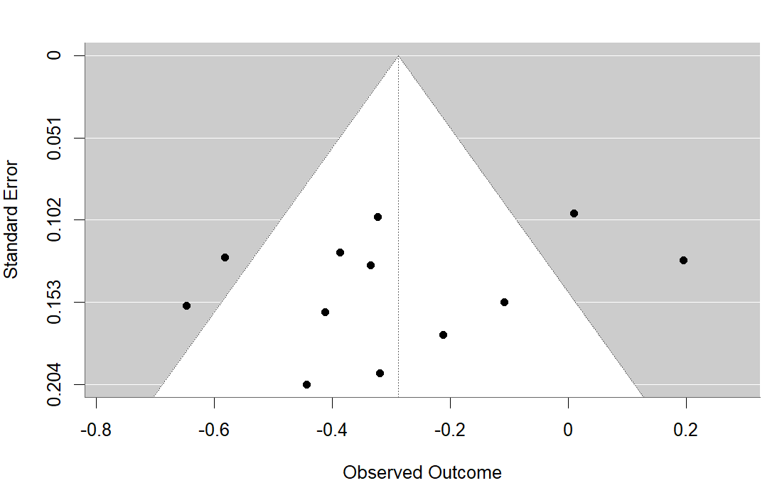
R output. # studies.csv, one row per trial in a meta-analysis. import pandas as pd, matplotlib.pyplot as plt d = pd.read_csv("https://paulinadelmundomd.com/data/meta/studies.csv") plt.scatter(d.yi, d.sei); plt.gca().invert_yaxis() plt.xlabel("log OR"); plt.ylabel("standard error"); plt.title("Funnel plot (Python)") plt.show()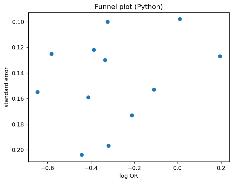
Python output.
G
- Generalized linear mixed model (GLMM)
- A mixed model for non-normal outcomes: cluster-level random effects are added to a generalized linear model, for example logistic or Poisson regression with a random intercept per group. Its coefficients are subject-specific (conditional), so under a nonlinear link they differ from the population-average estimates a marginal model or GEE reports. The likelihood involves an integral over the random effects with no closed form, so it needs approximate fitting. in the pathway → · Dohoo, Martin & Stryhn, 2012
- Geographic information system (GIS)
- Software for storing, linking, analysing, and mapping geo-referenced data, pairing spatial features (points, lines, polygons) with attribute tables so locations can be queried and visualised together. Spatial data come in two forms: vector (discrete points, lines, and polygons, good for boundaries and addresses) and raster (a grid of cells each holding a value, good for continuous surfaces like elevation or pollution). It is the basic platform for disease mapping and spatial analysis. in the pathway → · Dohoo, Martin & Stryhn, 2012
- G-estimation
- A g-method for confounding that changes over time, where past treatment affects future confounders which in turn affect later treatment. It fits a structural nested model (a model for the treatment effect at each time step) rather than adjusting in the usual way, which would bias the estimate. in the pathway →
- G-formula
-
G-computation: modeling the outcome under each treatment and averaging over the covariate distribution. in the pathway →
\[E[Y(a)] = \sum_x E[Y \mid A=a,\, X=x]\, P(X=x)\]
where fit an outcome model, predict under treatment level \(a\) for everyone, and average over the covariate distribution \(P(X)\) (standardization).
Standardizing over the covariate distribution gives an estimated effect of about -0.041 on the risk scale, roughly 4 fewer events per 100 had everyone been exposed versus not. It relies on a correct outcome model and no unmeasured confounding.
# OMOP cohort: standardization (g-formula) - average risk if all exposed vs none.
# cohort.csv, one row per person: age = age in years; sex = sex (M/F); comorbidity = comorbidity count; exposed = drug exposure, 0/1; outcome = outcome condition, 0/1.
coh <- read.csv("https://paulinadelmundomd.com/data/omop/cohort.csv")
fit <- glm(outcome ~ exposed + age + sex + comorbidity, data = coh, family = binomial)
mean(predict(fit, transform(coh, exposed=1), type="response")) -
  mean(predict(fit, transform(coh, exposed=0), type="response"))   # standardized RD
Result:
[1] -0.04110019# OMOP cohort: standardization (g-formula) - average risk if all exposed vs none. # cohort.csv, one row per person: age = age in years; sex = sex (M/F); comorbidity = comorbidity count; exposed = drug exposure, 0/1; outcome = outcome condition, 0/1. import pandas as pd, statsmodels.formula.api as smf coh = pd.read_csv("https://paulinadelmundomd.com/data/omop/cohort.csv") fit = smf.logit("outcome ~ exposed + age + C(sex) + comorbidity", coh).fit(disp=0) r1 = fit.predict(coh.assign(exposed=1)); r0 = fit.predict(coh.assign(exposed=0)) r1.mean() - r0.mean() # standardized (g-formula) risk differenceResult:
-0.04110019376073182 - Gate question
- A question that routes a respondent past items that do not apply, creating by-design blanks. in the pathway →
- Gatekeeping procedure
- A hierarchical procedure ordering trial hypotheses and spending alpha down the sequence, testing a secondary endpoint only if the primary won. in the pathway →
- GDPR
- The General Data Protection Regulation, the European regulation imposing a stricter consent-and-purpose regime on personal data than US rules. in the pathway → · EUR-Lex: GDPR (Regulation (EU) 2016/679) ↗
- GEE
-
Generalized estimating equations, used for clustered or repeated measures. in the pathway →
The population-averaged dose effect is about -0.014 per unit, with the working correlation absorbing the repeated measures within subjects. GEE targets the average across the population, not any one subject’s trajectory.
# CDISC ADaM ADQS: repeated ADAS-Cog over visits, GEE with exchangeable working correlation.
# adqs.csv, one row per subject-visit: USUBJID = subject id; AVISITN = visit number; AVAL = score at that visit; TRTPN = treatment code.
library(geepack)
adqs <- read.csv("https://paulinadelmundomd.com/data/cdisc/adqs.csv")
geeglm(AVAL ~ AVISITN + TRTPN, id = USUBJID, data = adqs, corstr = "exchangeable")
Result:
Call:
geeglm(formula = AVAL ~ AVISITN + TRTPN, data = adqs, id = USUBJID,
    corstr = "exchangeable")

Coefficients:
(Intercept)     AVISITN       TRTPN
25.55843502 -0.03079232 -0.01437352

Degrees of Freedom: 1016 Total (i.e. Null);  1013 Residual

Scale Link:                   identity
Estimated Scale Parameters:  [1] 76.05943

Correlation:  Structure = exchangeable    Link = identity
Estimated Correlation Parameters:
        alpha
-0.0009852217
... (truncated)
# CDISC ADaM ADQS: repeated ADAS-Cog over visits, GEE with exchangeable working correlation. # adqs.csv, one row per subject-visit: USUBJID = subject id; AVISITN = visit number; AVAL = score at that visit; TRTPN = treatment code. import pandas as pd, statsmodels.formula.api as smf, statsmodels.api as sm adqs = pd.read_csv("https://paulinadelmundomd.com/data/cdisc/adqs.csv") smf.gee("AVAL ~ AVISITN + TRTPN", groups="USUBJID", data=adqs, cov_struct=sm.cov_struct.Exchangeable()).fit().summary()Result:
GEE Regression Results =================================================================================== Dep. Variable: AVAL No. Observations: 1016 Model: GEE No. clusters: 254 Method: Generalized Min. cluster size: 4 Estimating Equations Max. cluster size: 4 Family: Gaussian Mean cluster size: 4.0 Dependence structure: Exchangeable Num. iterations: 2 Scale: 76.285 Covariance type: robust ============================================================================== coef std err z P>|z| [0.025 0.975] ------------------------------------------------------------------------------ Intercept 25.5584 0.781 32.712 0.000 24.027 27.090 AVISITN -0.0308 0.009 -3.332 0.001 -0.049 -0.013 TRTPN -0.0144 0.015 -0.944 0.345 -0.044 0.015 ============================================================================== Skew: -0.1082 Kurtosis: -0.1526 ... (truncated) - Generalizability and transportability
- Generalizability asks whether the study sample represents the target population; transportability formalizes when an estimate can be carried to a different population. in the pathway → · Dohoo, Martin & Stryhn, 2012
- Generalized additive models
- Models that extend splines to fit smooth nonlinear predictor effects. in the pathway → \[g(\mathbb{E}[Y]) = \beta_0 + \sum_j f_j(x_j)\] where each \(f_j\) is a smooth function and \(g\) the link.
- Gibbs sampling
- An MCMC algorithm that samples the joint posterior by drawing each parameter in turn from its full conditional distribution given the current values of the others, cycling through them. It applies when those full conditionals are known and easy to sample from. in the pathway → \[\theta_j^{(t+1)} \sim p\big(\theta_j \mid \theta_{-j}^{(t)},\, x\big)\] where each parameter is drawn from its full conditional given the current values of the others.
- GLM
-
A generalized linear model: a choice of outcome distribution plus a link function. in the pathway →
\[g\big(E[Y \mid X]\big) = X\beta\]
where the link function \(g\) connects the mean of \(Y\) to the linear predictor \(X\beta\); choosing \(g\) and the outcome distribution gives linear, logistic, or Poisson regression.
Each comorbidity multiplies the expected visit count by about 1.03 (Poisson, log link). A GLM generalizes ordinary regression to non-normal outcomes by pairing a distribution with a link function; logistic regression is the binomial-with-logit member of the family.
# OMOP cohort: a generalized linear model -- here Poisson with a log link for a
# count outcome. exp(coef) is the rate ratio, the multiplicative change in the
# expected visit count per unit predictor. cohort.csv: n_visits, age, comorbidity.
coh <- read.csv("https://paulinadelmundomd.com/data/omop/cohort.csv")
unname(exp(coef(glm(n_visits ~ age + comorbidity, poisson, coh))["comorbidity"]))   # rate ratio
Result:
[1] 1.026621# OMOP cohort: a generalized linear model -- here Poisson with a log link for a # count outcome. exp(coef) is the rate ratio, the multiplicative change in the # expected visit count per unit predictor. cohort.csv: n_visits, age, comorbidity. import pandas as pd, numpy as np, statsmodels.formula.api as smf, statsmodels.api as sm coh = pd.read_csv("https://paulinadelmundomd.com/data/omop/cohort.csv") m = smf.glm("n_visits ~ age + comorbidity", data=coh, family=sm.families.Poisson()).fit() float(np.exp(m.params["comorbidity"])) # rate ratioResult:
1.026621183684227 - Gold standard
- A reference test or procedure taken to be perfectly accurate, calling every truly diseased person positive and every healthy one negative. True gold standards are rare (both the assay and the underlying biology are imperfect), which is why sensitivity and specificity are often estimated against an imperfect reference, a composite reference standard, or no reference at all through latent class analysis. in the pathway → · Dohoo, Martin & Stryhn, 2012
- Good clinical practice
- The operational standard (ICH E6) making a trial’s data trustworthy through defined responsibilities, a followed protocol, source-data verification, and an audit trail. in the pathway → · ICH: E6 Good Clinical Practice ↗
- Grace period and permissible gap
- Allowed days between supplies before exposure is broken, and extra coverage past the last day of supply before discontinuation. in the pathway →
- GRADE
- Grading of Recommendations Assessment, Development and Evaluation, a system rating the certainty of a body of evidence, downgrading for risk of bias, inconsistency, indirectness, imprecision, and publication bias. in the pathway → · GRADE working group ↗
- Gradient boosting
-
An ensemble that grows trees in sequence, each one fitting the errors the earlier trees left behind, so the model keeps improving where it was previously wrong. in the pathway →
The boosted ensemble classifies held-out cases correctly about 66 to 70% of the time. Boosting often edges out a single tree, but it adds knobs (tree depth, learning rate, number of trees) that need tuning to avoid overfitting.
# OMOP cohort: gradient-boosted trees for the outcome.
# cohort.csv, one row per person: age = age in years; sex = sex (M/F); comorbidity = comorbidity count; n_visits = number of visits; outcome = outcome condition, 0/1.
library(gbm)
coh <- read.csv("https://paulinadelmundomd.com/data/omop/cohort.csv"); coh$sexN <- as.integer(coh$sex == "M")
set.seed(8); tr <- sample(nrow(coh), 0.7 * nrow(coh))
fit <- gbm(outcome ~ age + sexN + comorbidity + n_visits, data = coh[tr, ],
           distribution = "bernoulli", n.trees = 300,
           interaction.depth = 2, shrinkage = 0.05)
p <- predict(fit, coh[-tr, ], n.trees = 300, type = "response")
mean((p > 0.5) == coh$outcome[-tr])   # held-out accuracy
Result:
[1] 0.66# OMOP cohort: gradient-boosted trees for the outcome. # cohort.csv, one row per person: age = age in years; sex = sex (M/F); comorbidity = comorbidity count; n_visits = number of visits; outcome = outcome condition, 0/1. import pandas as pd from sklearn.ensemble import GradientBoostingClassifier from sklearn.model_selection import train_test_split coh = pd.read_csv("https://paulinadelmundomd.com/data/omop/cohort.csv"); coh["sexM"] = (coh["sex"] == "M").astype(int) X = coh[["age", "sexM", "comorbidity", "n_visits"]]; y = coh["outcome"] Xtr, Xte, ytr, yte = train_test_split(X, y, test_size=0.3, random_state=8) GradientBoostingClassifier(n_estimators=300, max_depth=2, learning_rate=0.05).fit(Xtr, ytr).score(Xte, yte) # held-out accuracyResult:
0.7033333333333334 - Gradient descent
-
An optimization that repeatedly steps the parameters in the direction that most reduces a loss, the workhorse for fitting models with no closed-form solution. in the pathway →
After 2,000 small steps the estimate settles at -0.79, the exact OLS slope, reached without ever solving the normal equations. Gradient descent is how models too large for a closed form (neural networks, the leaves of boosted trees) are actually fit; the learning rate and step count are the knobs.
# ACS counties: gradient descent recovering a regression slope by repeatedly
# stepping against the loss gradient. On standardized income vs poverty it
# converges to the OLS slope (which for standardized data is the correlation).
cty <- read.csv("https://paulinadelmundomd.com/data/acs/counties.csv")
x <- scale(cty$poverty_pct)[, 1]; y <- scale(cty$median_income)[, 1]; b <- 0
for (i in 1:2000) b <- b - 0.01 * (-2 / length(y)) * sum(x * (y - b * x))
b                               # slope after 2000 steps
Result:
[1] -0.7899105# ACS counties: gradient descent recovering a regression slope by repeatedly # stepping against the loss gradient. On standardized income vs poverty it # converges to the OLS slope (which for standardized data is the correlation). import pandas as pd cty = pd.read_csv("https://paulinadelmundomd.com/data/acs/counties.csv") z = lambda c: ((c - c.mean()) / c.std(ddof=1)).to_numpy() x = z(cty.poverty_pct); y = z(cty.median_income); b = 0.0 for _ in range(2000): b = b - 0.01 * (-2 / len(y)) * (x * (y - b * x)).sum() float(b) # slope after 2000 stepsResult:
-0.7899105371292215 - Grid search
-
Tuning hyperparameters by evaluating every combination on a predefined grid and keeping the best by cross-validated performance; simple but costly as the grid grows. in the pathway →
Five-fold CV picks cost=10 and gamma=0.1 as the best of the six combinations tried. Grid search only explores the values you list, so its winner is the best on the grid, not necessarily the global optimum.
# Cross-validated search over a 2-D grid of SVM hyperparameters (cost, gamma).
# cohort.csv, one row per person: age = age in years; sex = sex (M/F); comorbidity = comorbidity count; n_visits = number of visits; outcome = outcome condition, 0/1.
library(e1071)
coh <- read.csv("https://paulinadelmundomd.com/data/omop/cohort.csv"); coh$sexM <- as.integer(coh$sex == "M")
coh$outcome <- factor(coh$outcome); set.seed(7)
g <- tune(svm, outcome ~ age + sexM + comorbidity + n_visits, data = coh,
          ranges = list(cost = c(0.1, 1, 10), gamma = c(0.01, 0.1)))
g$best.parameters   # (cost, gamma) with the best CV performance
Result:
  cost gamma
6   10   0.1
# Cross-validated search over a 2-D grid of SVM hyperparameters (C, gamma). # cohort.csv, one row per person: age = age in years; sex = sex (M/F); comorbidity = comorbidity count; n_visits = number of visits; outcome = outcome condition, 0/1. import pandas as pd from sklearn.svm import SVC from sklearn.model_selection import GridSearchCV coh = pd.read_csv("https://paulinadelmundomd.com/data/omop/cohort.csv"); coh["sexM"] = (coh["sex"] == "M").astype(int) X = coh[["age", "sexM", "comorbidity", "n_visits"]]; y = coh["outcome"] gs = GridSearchCV(SVC(), {"C": [0.1, 1, 10], "gamma": [0.01, 0.1]}, cv=5).fit(X, y) gs.best_params_ # (C, gamma) with the best CV performanceResult:
{'C': 1, 'gamma': 0.01} - Gross costing
- Top-down costing that values a whole episode of care with one aggregate weight such as a DRG payment. in the pathway →
- Group-level testing
-
Classifying a whole group (a herd, household, or village) from tests on its members. Group sensitivity and specificity depend on the individual sensitivity and specificity, the within-group prevalence, the number tested, and how many positives are required to declare the group positive; for a one-positive rule, \(GSe = 1 - (1 - AP_{\text{pos}})^n\). Testing pooled specimens is a related cost-saving variant that trades some sensitivity (dilution) for covering more individuals. in the pathway → · Dohoo, Martin & Stryhn, 2012
Pooling makes detection nearly certain (0.999) when three infected members each have a 90% chance of testing positive, because only one needs to be caught. Group-level testing trades individual resolution for cheap, sensitive surveillance across herds, households, or wastewater.
# Group (pooled) testing: the herd sensitivity of calling a group positive when
# at least one of its d truly-infected members tests positive, given an
# individual test sensitivity Se: HSe = 1 - (1 - Se)^d. Here Se = 0.90, d = 3.
Se <- 0.90; d <- 3
1 - (1 - Se)^d                  # group (herd) sensitivity
Result:
[1] 0.999# Group (pooled) testing: the herd sensitivity of calling a group positive when # at least one of its d truly-infected members tests positive, given an # individual test sensitivity Se: HSe = 1 - (1 - Se)^d. Here Se = 0.90, d = 3. Se, d = 0.90, 3 1 - (1 - Se)**d # group (herd) sensitivityResult:
0.999 - Group-sequential design
- A design that pre-specifies interim analyses and spends the alpha across them with a stopping boundary. in the pathway →
H
- Half-cycle correction
- In a Markov cohort model, where a simulated group moves between health states in discrete cycles, a fix for the counting error from tallying membership only at cycle boundaries, since on average subjects transition partway through a cycle. in the pathway →
- Hamiltonian Monte Carlo
- A method for drawing samples from a hard-to-sample distribution by using its gradient (slope) to propose smart moves, so it explores far more efficiently in high dimensions than random-walk samplers. It is the engine behind the Stan software. in the pathway →
- Hawthorne effect
- A follow-up bias in which subjects change their behaviour simply because they know they are being studied, rather than because of the exposure. In an observational study the researcher is meant to observe, not alter, the usual course of events, but the act of asking about diet, housing, or habits can prompt participants to modify them. Complete and equal follow-up of the groups is the main defence. in the pathway → · Dohoo, Martin & Stryhn, 2012
- Hazard function
- The instantaneous rate of the event at time \(t\) among those still at risk, \(h(t)\), the engine of survival analysis. It ties to the survival function \(S(t)\), the probability of lasting past \(t\), and the cumulative hazard \(H(t)=\int_0^t h(u)\,du\) through \(S(t)=e^{-H(t)}\), so a rising, falling, bathtub, or flat hazard shapes the whole curve. The Kaplan-Meier estimator targets \(S(t)\) nonparametrically and the Nelson-Aalen estimator targets \(H(t)\); the Cox model models how covariates scale \(h(t)\). in the pathway → · Dohoo, Martin & Stryhn, 2012
- Hazard rate
-
The instantaneous form of an incidence rate: the theoretical limit of new cases per person-time as the interval shrinks to zero, \(h(t) = \lim_{\Delta t \to 0} I\). It is the quantity modeled in survival analysis and compared by proportional-hazards methods, and can be defined cause by cause. in the pathway → · Dohoo, Martin & Stryhn, 2012
The crude hazard rate is 0.016 events per unit time, the instantaneous form of an incidence rate. A Kaplan-Meier or Cox model lets the hazard vary over time rather than collapsing it to this single average.
# CDISC ADaM ADTTE: the crude hazard rate, events per unit person-time --
# total events over total observed time. adtte.csv: AVAL = time, CNSR = 1 if censored.
a <- read.csv("https://paulinadelmundomd.com/data/cdisc/adtte.csv")
sum(1 - a$CNSR) / sum(a$AVAL)   # events per person-time
Result:
[1] 0.01609316# CDISC ADaM ADTTE: the crude hazard rate, events per unit person-time -- # total events over total observed time. adtte.csv: AVAL = time, CNSR = 1 if censored. import pandas as pd a = pd.read_csv("https://paulinadelmundomd.com/data/cdisc/adtte.csv") float((1 - a.CNSR).sum() / a.AVAL.sum()) # events per person-timeResult:
0.016093160752027186 - Hazard ratios and non-proportional hazards
-
The ratio of the instantaneous event rates in two groups: 1 means equal risk at every moment, 1.5 a 50% higher hazard, and below 1 protective. It assumes a constant effect on instantaneous risk over time; when that fails, the single ratio becomes a censoring-dependent weighted average. A subtler problem is built in: the hazard at time \(t\) is conditional on having survived to \(t\), so as follow-up lengthens the still-susceptible members of the exposed group are depleted and the ratio drifts toward the null, which leaves even the reported average hazard ratio dependent on how long the study ran. in the pathway → · Dohoo, Martin & Stryhn, 2012
\[\text{HR} = \dfrac{h_1(t)}{h_0(t)}\]
where \(h_1(t)\) and \(h_0(t)\) are the hazards in the two groups at time \(t\); under proportional hazards the ratio is constant over time.
The hazard ratio is 0.99 – essentially no treatment effect on the event rate. A single HR assumes proportional hazards, a constant ratio at every time. When that fails (delayed effects, crossing curves) the HR becomes a hard-to-read time average, and RMST or a milestone analysis is clearer.
# CDISC ADaM ADTTE: the hazard ratio for treatment from a Cox proportional-
# hazards model. exp(coef) is the ratio of instantaneous event rates.
# adtte.csv: AVAL = time, CNSR = 1 if censored, TRTPN = arm.
library(survival)
a <- read.csv("https://paulinadelmundomd.com/data/cdisc/adtte.csv")
unname(exp(coef(coxph(Surv(AVAL, 1 - CNSR) ~ TRTPN, a))))   # hazard ratio
Result:
[1] 0.9916263# CDISC ADaM ADTTE: the hazard ratio for treatment from a Cox proportional- # hazards model. exp(coef) is the ratio of instantaneous event rates. # adtte.csv: AVAL = time, CNSR = 1 if censored, TRTPN = arm. import pandas as pd, numpy as np from lifelines import CoxPHFitter a = pd.read_csv("https://paulinadelmundomd.com/data/cdisc/adtte.csv").assign(event=lambda d: 1 - d.CNSR) cph = CoxPHFitter().fit(a[["AVAL", "event", "TRTPN"]], "AVAL", "event") float(np.exp(cph.params_["TRTPN"])) # hazard ratioResult:
0.991626269835074 - Health technology assessment and value frameworks
- A body weighing cost-effectiveness against clinical benefit, budget impact, and equity to reach a coverage or pricing verdict, run differently across health systems. in the pathway →
- Health-state utility
- A preference-based weight for a health state on a scale where 1 is full health and 0 is death, elicited from instruments like the EQ-5D or time-trade-off and standard-gamble methods. It supplies the quality weight in a QALY. in the pathway →
- Healthy-worker effect
- The tendency of an employed cohort to be healthier than the general population. in the pathway →
- Herd immunity
- The protection unvaccinated people gain when enough of those around them are immune that transmission cannot sustain itself; it is the population face of a vaccine’s indirect effect. Because vaccinated and unvaccinated subjects are not independent (formally, an assumption of no interference, part of SUTVA), a vaccine’s benefit exceeds its direct effect on recipients, and there is a critical vaccination fraction, often well below 100%, above which the agent is eliminated. It is why population vaccine efficacy depends on coverage, not on the vaccine alone. in the pathway → · Dohoo, Martin & Stryhn, 2012
- Herd-immunity threshold
-
The fraction of a population that must be immune for herd immunity to halt sustained transmission, \(1-1/R_0\) in a well-mixed population. A pathogen with \(R_0\) of 5 needs about 80% immune; a more transmissible one needs more, which is why measles demands such high coverage. Real thresholds run higher when mixing is uneven or immunity is imperfect or wanes, so the simple formula is a floor, not a guarantee. in the pathway → · Dohoo, Martin & Stryhn, 2012
At R0 = 3, about 67% of the population must be immune before each case infects fewer than one other on average and transmission dies out. A higher R0 (measles near 15) pushes the threshold above 90%, which is why measles demands such high vaccination coverage.
# Herd-immunity threshold: the immune fraction needed to halt sustained
# transmission, HIT = 1 - 1/R0. Here a pathogen with basic reproduction number 3.
R0 <- 3
1 - 1 / R0                      # herd-immunity threshold
Result:
[1] 0.6666667# Herd-immunity threshold: the immune fraction needed to halt sustained # transmission, HIT = 1 - 1/R0. Here a pathogen with basic reproduction number 3. R0 = 3 1 - 1 / R0 # herd-immunity thresholdResult:
0.6666666666666667 - Heterogeneity
-
The degree to which studies’ results actually disagree beyond chance, which decides whether a pooled number is informative or a fiction. in the pathway →
Q is 37.8, I-squared about 71%, and tau-squared about 0.045, so roughly 71% of the variation across studies reflects true differences in effect rather than chance. That is substantial heterogeneity, which is why a random-effects pooling (carrying this tau-squared) is the honest summary here rather than a fixed-effect one.
# metafor reports Q, I^2 and tau^2 (DerSimonian-Laird here, matching the Python).
# studies.csv, one row per trial: yi = effect estimate (log OR); sei = standard error of yi.
library(metafor)
d <- read.csv("https://paulinadelmundomd.com/data/meta/studies.csv")
res <- rma(yi, sei = sei, data = d, method = "DL")
c(Q = res$QE, I2 = res$I2, tau2 = res$tau2)
Result:
         Q         I2       tau2
37.8039176 70.9024866  0.0449079
# studies.csv, one row per trial: yi = effect estimate (log OR); sei = standard error of yi. import numpy as np, pandas as pd d = pd.read_csv("https://paulinadelmundomd.com/data/meta/studies.csv") yi = d.yi.values; vi = d.sei.values**2; k = len(yi); w = 1/vi Q = (w*(yi - (w*yi).sum()/w.sum())**2).sum() tau2 = max(0, (Q-(k-1)) / (w.sum() - (w**2).sum()/w.sum())) # DerSimonian-Laird I2 = max(0, (Q-(k-1))/Q) print("Q=%.2f I2=%.1f%% tau2=%.4f" % (Q, 100*I2, tau2))Result:
Q=37.80 I2=70.9% tau2=0.0449 - Heteroscedasticity
-
Non-constant residual variance, where the spread of the errors changes across the range of the predictors. It leaves the coefficients unbiased but makes the standard errors wrong, so tests and intervals can mislead. Read it from a residual-versus-fitted plot, confirm with Breusch-Pagan or White. in the pathway →
The BP statistic (0.18 on 2 df, chi-square) is far from significant, so the residual variance looks constant across these predictors. When it isn’t, ordinary standard errors mislead, and robust (sandwich) errors or a variance-stabilizing transform are the fix.
# ACS counties: a Breusch-Pagan test for heteroscedasticity -- regress the
# squared residuals on the predictors; the LM statistic is n times that
# auxiliary R-squared, large when the error spread varies with the predictors.
# counties.csv: median_income, poverty_pct, bachelors_pct.
cty <- read.csv("https://paulinadelmundomd.com/data/acs/counties.csv")
e2 <- resid(lm(median_income ~ poverty_pct + bachelors_pct, cty))^2
nrow(cty) * summary(lm(e2 ~ cty$poverty_pct + cty$bachelors_pct))$r.squared   # BP LM statistic
Result:
[1] 0.1791949# ACS counties: a Breusch-Pagan test for heteroscedasticity -- regress the # squared residuals on the predictors; the LM statistic is n times that # auxiliary R-squared, large when the error spread varies with the predictors. # counties.csv: median_income, poverty_pct, bachelors_pct. import pandas as pd, statsmodels.formula.api as smf cty = pd.read_csv("https://paulinadelmundomd.com/data/acs/counties.csv") cty["e2"] = smf.ols("median_income ~ poverty_pct + bachelors_pct", cty).fit().resid**2 float(len(cty) * smf.ols("e2 ~ poverty_pct + bachelors_pct", cty).fit().rsquared) # BP LMResult:
0.17919492794060443 - Hierarchical Bayesian models
- Multilevel models that estimate each group’s parameter while sharing a common prior, pulling estimates toward the mean. in the pathway →
- Hierarchical clustering
-
A clustering method building a nested tree of groupings without fixing the number of clusters in advance. in the pathway →
Cutting the dendrogram yields four groups, and the labels show which county lands in each. Where you cut sets the number of clusters; the method does not decide it for you.
# ACS counties (a sample): hierarchical clustering of socioeconomic profiles.
# counties.csv, one row per US county: median_income = median household income; poverty_pct = percent in poverty; bachelors_pct = percent with a bachelor degree.
acs <- read.csv("https://paulinadelmundomd.com/data/acs/counties.csv")[1:60, ]
X <- scale(acs[c("median_income","poverty_pct","bachelors_pct")])
cutree(hclust(dist(X)), k = 4)   # 4-cluster assignment
Result:
1 2 3 4 5 6 7 8 9 10 11 12 13 14 15 16 17 18 19 20 21 22 23 24 25 26 1 1 2 3 2 1 1 3 2 2 2 2 2 2 2 2 4 4 1 2 1 2 1 4 4 4 27 28 29 30 31 32 33 34 35 36 37 38 39 40 41 42 43 44 45 46 47 48 49 50 51 52 2 2 2 4 2 4 3 2 4 2 1 2 4 2 1 4 4 4 4 2 2 4 4 1 2 1 53 54 55 56 57 58 59 60 1 2 2 1 2 4 4 1# ACS counties (a sample): hierarchical clustering of socioeconomic profiles. # counties.csv, one row per US county: median_income = median household income; poverty_pct = percent in poverty; bachelors_pct = percent with a bachelor degree. import pandas as pd; from scipy.cluster.hierarchy import linkage, fcluster; from sklearn.preprocessing import scale acs = pd.read_csv("https://paulinadelmundomd.com/data/acs/counties.csv").head(60) X = scale(acs[["median_income","poverty_pct","bachelors_pct"]]) fcluster(linkage(X, "ward"), t=4, criterion="maxclust")Result:
[2 2 3 4 3 2 2 4 4 4 3 4 3 3 4 3 1 1 2 4 2 4 2 1 1 1 3 4 4 1 4 1 4 3 1 4 2 3 1 3 2 1 1 1 1 3 4 1 1 2 3 2 2 4 4 2 3 1 1 2] - High-dimensional propensity score (hdPS)
- An algorithm that screens thousands of claims codes and selects the ones that behave like confounders, so it catches confounders you never thought to measure and feeds them to the propensity-score model automatically. in the pathway →
- Hill criteria
- Bradford Hill’s nine viewpoints for judging whether an association is causal: strength, consistency across studies, specificity, temporality (cause precedes effect, the one near-necessary criterion), a biological gradient (dose-response), plausibility, coherence, experimental evidence, and analogy. Hill offered them as aids to judgement, not a checklist to tick off; only temporality is truly required, while the others raise or lower confidence. They remain the informal backbone of causal argument from observational data, complementing formal tools like causal diagrams and the potential-outcomes framework. in the pathway → · Dohoo, Martin & Stryhn, 2012
- HIPAA
- The Health Insurance Portability and Accountability Act, the US law governing identifiable health information, which a dataset must satisfy through de-identification before sharing for research. in the pathway → · HHS: The HIPAA Privacy Rule ↗
- Historical control
- A before-and-after comparison that contrasts outcomes after an intervention with recorded outcomes from an earlier period rather than a concurrent randomized arm. It is valid only under stringent conditions rarely all met: a predictable outcome, complete and accurate historical records, unchanged diagnostic criteria, and no secular change in the subjects’ environment. It also precludes blinding, so it sits well below a concurrent RCT in the evidence hierarchy. in the pathway → · Dohoo, Martin & Stryhn, 2012
- Holm’s procedure
- A step-down procedure controlling the family-wise error rate with more power than Bonferroni. in the pathway → \[\text{reject } H_{(i)} \text{ while } p_{(i)} \le \dfrac{\alpha}{m - i + 1}\] where \(p_{(i)}\) are the ordered p-values and \(m\) the number of tests.
- Homogeneity check
-
The test before pooling for whether stratum-specific estimates differ by more than noise, which would indicate effect modification. in the pathway →
\[\hat H = \sum_{g=1}^{G}\dfrac{(O_g - E_g)^{2}}{E_g\,(1 - E_g/n_g)}\]
where \(O_g\), \(E_g\), \(n_g\) are observed events, expected events, and count in risk group \(g\); \(\hat H \sim \chi^{2}_{G-1}\).
Q = 37.8 on 11 df (12 studies) far exceeds its expectation of 11, signaling real between-study heterogeneity: the studies are not all estimating one common effect, which argues for a random-effects over a fixed-effect model. Q feeds directly into the I-squared statistic.
# Meta-analysis studies: Cochran's Q, the homogeneity test before pooling -- # the inverse-variance weighted sum of squared deviations of each study from the # pooled effect. studies.csv: yi = log odds ratio, sei = its standard error. st <- read.csv("https://paulinadelmundomd.com/data/meta/studies.csv") w <- 1 / st$sei^2; pooled <- sum(w * st$yi) / sum(w) sum(w * (st$yi - pooled)^2) # Cochran's QResult:
[1] 37.80392# Meta-analysis studies: Cochran's Q, the homogeneity test before pooling -- # the inverse-variance weighted sum of squared deviations of each study from the # pooled effect. studies.csv: yi = log odds ratio, sei = its standard error. import pandas as pd st = pd.read_csv("https://paulinadelmundomd.com/data/meta/studies.csv") w = 1 / st.sei**2; pooled = (w * st.yi).sum() / w.sum() float((w * (st.yi - pooled)**2).sum()) # Cochran's QResult:
37.80391763926621 - Hosmer-Lemeshow test
-
A goodness-of-fit test for logistic regression: subjects are ranked by predicted probability, split into (usually ten) groups, and observed versus expected event counts are compared with a chi-squared statistic; a small p-value flags poor calibration. It is easy to run but depends on the number of groups, has low power in small samples, and can reject trivially in very large ones, so it is best read alongside a calibration plot. in the pathway → · Dohoo, Martin & Stryhn, 2012
HL = 6.23 on 8 df (p about 0.6) shows no evidence of poor calibration: observed and predicted event counts agree across risk deciles. The test is sensitive to the number of groups and to sample size, so it is read alongside a calibration plot.
# OMOP cohort: the Hosmer-Lemeshow goodness-of-fit statistic for a logistic # model -- split subjects into ten predicted-risk deciles and compare observed # to expected events, summed as a chi-square. cohort.csv: outcome, predictors. coh <- read.csv("https://paulinadelmundomd.com/data/omop/cohort.csv") p <- predict(glm(outcome ~ age + comorbidity + n_visits, binomial, coh), type = "response") y <- coh$outcome; n <- length(p); g <- integer(n); g[order(p)] <- floor((0:(n-1)) / n * 10) HL <- 0 for (j in 0:9) { i <- g == j; O <- sum(y[i]); E <- sum(p[i]); nj <- sum(i) HL <- HL + (O - E)^2 / E + ((nj - O) - (nj - E))^2 / (nj - E) } HL # Hosmer-Lemeshow statisticResult:
[1] 6.229821# OMOP cohort: the Hosmer-Lemeshow goodness-of-fit statistic for a logistic # model -- split subjects into ten predicted-risk deciles and compare observed # to expected events, summed as a chi-square. cohort.csv: outcome, predictors. import pandas as pd, numpy as np, statsmodels.formula.api as smf coh = pd.read_csv("https://paulinadelmundomd.com/data/omop/cohort.csv") p = np.asarray(smf.logit("outcome ~ age + comorbidity + n_visits", coh).fit(disp=0).predict()) y = coh.outcome.to_numpy(); n = len(p) g = np.empty(n, int); g[np.argsort(p, kind="stable")] = np.arange(n) * 10 // n HL = 0.0 for j in range(10): i = g == j; O = y[i].sum(); E = p[i].sum(); nj = i.sum() HL += (O - E)**2 / E + ((nj - O) - (nj - E))**2 / (nj - E) float(HL) # Hosmer-Lemeshow statisticResult:
6.229820676192902 - Human-capital approach
- Valuing lost productivity by counting all earnings foregone to illness. in the pathway →
- Hurdle model
- A two-part model for count data with many zeros: one part predicts whether the count clears zero at all, the second predicts how large it is once it does. in the pathway →
- Hypergeometric distribution
-
The distribution of the number of successes drawn without replacement from a finite population, which is what governs a 2x2 table’s cell counts once its margins are fixed. It gives the exact probability of every table with those margins, and summing the ones no more likely than the table observed is Fisher’s exact test; it also underlies exact intervals for an odds ratio. in the pathway → · Dohoo, Martin & Stryhn, 2012
The chance is 0.21. Unlike the binomial, the hypergeometric draws without replacement, so each draw changes the remaining pool; it underlies Fisher’s exact test, which enumerates the tables consistent with fixed margins.
# The hypergeometric probability of drawing exactly 2 successes in 5 draws # without replacement from a population of 50 holding 10 successes -- the # sampling-without-replacement analogue of the binomial that Fisher's exact rests on. dhyper(2, 10, 40, 5) # P(exactly 2 successes)Result:
[1] 0.2098397# The hypergeometric probability of drawing exactly 2 successes in 5 draws # without replacement from a population of 50 holding 10 successes -- the # sampling-without-replacement analogue of the binomial that Fisher's exact rests on. from scipy import stats float(stats.hypergeom.pmf(2, 50, 10, 5)) # P(exactly 2 successes)Result:
0.2098397175706545 - Hyperparameter
-
A setting that governs how a model is fit rather than being learned from the data, such as a penalty strength, tree depth, or number of clusters, usually chosen by cross-validation. in the pathway →
Accuracy climbs from 0.67 at k=3 to 0.70 at k=31, so larger neighbourhoods smooth out noise here. The best value is data-specific, which is exactly why hyperparameters are tuned rather than fixed.
# Sweep one hyperparameter (k in kNN) and watch held-out accuracy move. # cohort.csv, one row per person: age = age in years; sex = sex (M/F); comorbidity = comorbidity count; n_visits = number of visits; outcome = outcome condition, 0/1. library(class) coh <- read.csv("https://paulinadelmundomd.com/data/omop/cohort.csv"); coh$sexM <- as.integer(coh$sex == "M") X <- scale(coh[, c("age", "sexM", "comorbidity", "n_visits")]) set.seed(6); tr <- sample(nrow(coh), 0.7 * nrow(coh)) acc <- sapply(c(3, 5, 11, 21, 31), function(k) mean(knn(X[tr, ], X[-tr, ], coh$outcome[tr], k = k) == coh$outcome[-tr])) setNames(round(acc, 3), c(3, 5, 11, 21, 31)) # accuracy vs the value of kResult:
3 5 11 21 31 0.667 0.640 0.687 0.697 0.703# Sweep one hyperparameter (k in kNN) and watch held-out accuracy move. # cohort.csv, one row per person: age = age in years; sex = sex (M/F); comorbidity = comorbidity count; n_visits = number of visits; outcome = outcome condition, 0/1. import pandas as pd from sklearn.neighbors import KNeighborsClassifier from sklearn.preprocessing import StandardScaler from sklearn.model_selection import train_test_split coh = pd.read_csv("https://paulinadelmundomd.com/data/omop/cohort.csv"); coh["sexM"] = (coh["sex"] == "M").astype(int) X = StandardScaler().fit_transform(coh[["age", "sexM", "comorbidity", "n_visits"]]); y = coh["outcome"] Xtr, Xte, ytr, yte = train_test_split(X, y, test_size=0.3, random_state=6) {k: round(KNeighborsClassifier(k).fit(Xtr, ytr).score(Xte, yte), 3) for k in [3, 5, 11, 21, 31]}Result:
{3: 0.713, 5: 0.703, 11: 0.743, 21: 0.717, 31: 0.743} - Hypothetical strategy
- One way of handling an intercurrent event (something like treatment switching or death that disrupts the intended comparison): estimate the outcome that would have occurred had the event not happened. in the pathway →
I
- Incidence from prevalence
-
Recovering an incidence estimate from cross-sectional data, which by itself measures only prevalence. The simplest route is two surveys run before and after a period, since the change between them is population-level incidence. For a long-lasting condition that barely affects mortality, age-specific prevalence at two ages \(n\) years apart gives \(I_a = 1 - \left[1 - \dfrac{P_{a+n} - P_a}{1 - P_a}\right]^{1/n}\). in the pathway → · Dohoo, Martin & Stryhn, 2012
About 0.022 new cases per person-year reproduce a 10% prevalence when cases last 5 years. The relation holds only in a steady state (stable incidence and duration); it is why prevalence rises with either more new cases or longer-lasting disease.
# Recovering incidence from cross-sectional prevalence for a condition in steady # state: I = P / (D * (1 - P)), with P the prevalence and D the mean duration. # Here a 10%-prevalent condition lasting 5 years on average. P <- 0.10; D <- 5 P / (D * (1 - P)) # incidence rateResult:
[1] 0.02222222# Recovering incidence from cross-sectional prevalence for a condition in steady # state: I = P / (D * (1 - P)), with P the prevalence and D the mean duration. # Here a 10%-prevalent condition lasting 5 years on average. P, D = 0.10, 5 P / (D * (1 - P)) # incidence rateResult:
0.022222222222222223 - Incidence rate difference
-
The absolute measure on the rate scale, \(\text{ID} = a_1/t_1 - a_0/t_0\): the extra cases per unit of person-time that exposure adds. Its variance follows directly, \(\text{var}(\text{ID}) = a_1/t_1^2 + a_0/t_0^2\), so its interval is the plain \(\text{ID} \pm Z_\alpha\sqrt{\text{var}}\) rather than one built on the log scale. The rate-scale counterpart of the risk difference. in the pathway → · Dohoo, Martin & Stryhn, 2012
The extra 0.00018 events per person-year is the rate-scale absolute measure: the excess cases attributable to exposure per unit person-time. Its reciprocal is a number-needed-to-treat expressed in person-time.
# OMOP cohort: the incidence rate difference, the absolute gap in event rate per # person-time between exposed and unexposed. cohort.csv: exposed, outcome, followup_years. coh <- read.csv("https://paulinadelmundomd.com/data/omop/cohort.csv") re <- sum(coh$outcome[coh$exposed == 1]) / sum(coh$followup_years[coh$exposed == 1]) ru <- sum(coh$outcome[coh$exposed == 0]) / sum(coh$followup_years[coh$exposed == 0]) re - ru # incidence rate differenceResult:
[1] 0.0001809848# OMOP cohort: the incidence rate difference, the absolute gap in event rate per # person-time between exposed and unexposed. cohort.csv: exposed, outcome, followup_years. import pandas as pd coh = pd.read_csv("https://paulinadelmundomd.com/data/omop/cohort.csv") re = coh.outcome[coh.exposed == 1].sum() / coh.followup_years[coh.exposed == 1].sum() ru = coh.outcome[coh.exposed == 0].sum() / coh.followup_years[coh.exposed == 0].sum() float(re - ru) # incidence rate differenceResult:
0.00018098481710372184 - Incidence rate ratio
-
The relative measure on the rate scale: the incidence rate among the exposed divided by the rate among the unexposed, \(\text{IR} = \dfrac{a_1/t_1}{a_0/t_0}\), where \(t\) is person-time. It can only be formed where a rate exists (a cohort study), and is sometimes called the incidence density ratio. As with other ratios, 1 is the null, below 1 protective, above 1 harmful. in the pathway → · Dohoo, Martin & Stryhn, 2012
The exposed have a 1.04-fold event rate per person-time. Unlike the risk ratio, the rate ratio carries person-time in its denominator, so it handles varying follow-up and is the natural measure for open cohorts and Poisson or Cox models.
# OMOP cohort: the incidence rate ratio, the event rate per person-time among # the exposed over the unexposed. cohort.csv: exposed, outcome, followup_years. coh <- read.csv("https://paulinadelmundomd.com/data/omop/cohort.csv") re <- sum(coh$outcome[coh$exposed == 1]) / sum(coh$followup_years[coh$exposed == 1]) ru <- sum(coh$outcome[coh$exposed == 0]) / sum(coh$followup_years[coh$exposed == 0]) re / ru # incidence rate ratioResult:
[1] 1.037495# OMOP cohort: the incidence rate ratio, the event rate per person-time among # the exposed over the unexposed. cohort.csv: exposed, outcome, followup_years. import pandas as pd coh = pd.read_csv("https://paulinadelmundomd.com/data/omop/cohort.csv") re = coh.outcome[coh.exposed == 1].sum() / coh.followup_years[coh.exposed == 1].sum() ru = coh.outcome[coh.exposed == 0].sum() / coh.followup_years[coh.exposed == 0].sum() float(re / ru) # incidence rate ratioResult:
1.0374954722097873 - Incident times
- The times at which incident cases occur, usually measured as elapsed time since a reference event (days from surgery to a recurrence). They are the raw material of survival analysis and the Kaplan-Meier estimator, rather than being collapsed into a single rate. in the pathway → · Dohoo, Martin & Stryhn, 2012
- Incubation period
- The time from infection to the onset of symptoms, distinct from the latent period, which runs from infection to the onset of infectiousness. When the latent period is shorter than the incubation period, people transmit before they feel ill, frustrating symptom-based control; when longer, isolating symptomatic cases works well. Its distribution sets quarantine lengths and helps back-calculate likely exposure times. in the pathway → · Dohoo, Martin & Stryhn, 2012
- Independence of irrelevant alternatives (IIA)
- An assumption of the multinomial logistic model: the odds between any two outcome categories do not depend on which other categories are available. It can fail when some options are close substitutes, so adding or removing one distorts the others (the classic red-bus/blue-bus problem), biasing the estimates. A Hausman-McFadden test checks it; nested or alternative-specific models relax it. in the pathway → · Dohoo, Martin & Stryhn, 2012
- Indirect standardization
-
The complement to direct standardization, used when a population’s own stratum-specific rates are unstable or unavailable: apply a reference population’s rates to your population’s structure for the expected count \(E = \sum_j T_j I_{sj}\), then form the standardized mortality ratio \(\text{SMR} = O/E\) and the standardized rate \(I_s \times \text{SMR}\). See age-standardization. in the pathway → · Dohoo, Martin & Stryhn, 2012
The SMR of 0.95 means the exposed had about 5% fewer events than expected from the whole cohort’s age-specific rates applied to their age mix. Indirect standardization is used when a group’s own stratum rates are unstable or unavailable, needing only its age structure and totals.
# OMOP cohort: indirect standardization -- apply the whole-cohort age-specific # rates to the exposed group's age structure for expected events, then form the # standardized ratio (SMR) of observed to expected. cohort.csv: age, exposed, outcome. coh <- read.csv("https://paulinadelmundomd.com/data/omop/cohort.csv") coh$ageg <- cut(coh$age, c(0, 40, 55, 70, Inf)); sr <- tapply(coh$outcome, coh$ageg, mean) ex <- coh[coh$exposed == 1, ]; expc <- tapply(ex$outcome, ex$ageg, length) sum(ex$outcome) / sum(expc * sr[names(expc)]) # SMR = observed / expectedResult:
[1] 0.948472# OMOP cohort: indirect standardization -- apply the whole-cohort age-specific # rates to the exposed group's age structure for expected events, then form the # standardized ratio (SMR) of observed to expected. cohort.csv: age, exposed, outcome. import pandas as pd, numpy as np coh = pd.read_csv("https://paulinadelmundomd.com/data/omop/cohort.csv") coh["ageg"] = pd.cut(coh.age, [0, 40, 55, 70, np.inf]); sr = coh.groupby("ageg").outcome.mean() ex = coh[coh.exposed == 1]; expc = ex.groupby("ageg").size() float(ex.outcome.sum() / (expc * sr).sum()) # SMR = observed / expectedResult:
0.948472043391301 - Influence function
- A function measuring how much a single observation sways an estimator; a wide class of estimators equals the sample average of its (estimated) influence function plus vanishing error. The AIPW estimator is exactly the sample mean of the efficient influence function for the treatment effect, which is why it attains the semiparametric efficiency bound, the lowest variance achievable without extra parametric assumptions, when the nuisance models are right. in the pathway → · Tsiatis, 2006
- Influential observation
- A data point whose removal would appreciably change a fitted model, distinct from a mere outlier in the outcome. Leverage measures how unusual a point is in the predictor space (a large hat-value), while influence pairs high leverage with a large residual; Cook’s distance and DFITS summarise how far the coefficients or fitted values move when the point is dropped. A few influential points can drive an entire result, so they should be found and understood rather than reflexively deleted. in the pathway → · Dohoo, Martin & Stryhn, 2012
- Information bias
- The umbrella term for bias from mismeasuring the exposure, outcome, or covariates, whether as misclassification of categorical variables (described by sensitivity and specificity) or measurement error in continuous ones. It is one of the three master biases alongside selection bias and confounding. Its direction is not always intuitive: non-differential errors usually pull toward the null, but differential errors can push either way. in the pathway → · Dohoo, Martin & Stryhn, 2012
- Internal validity
- Whether a study got the right answer for its own source population, free of selection, information, and confounding (confounder) bias, before any question of generalizing arises. Most of study design and analysis is machinery for protecting it. in the pathway → · Dohoo, Martin & Stryhn, 2012
- Intracluster correlation coefficient (ICC)
-
The share of total outcome variance that lies between clusters rather than within them, \(\rho\), measuring how alike members of one group (family, clinic, school) are. It inflates the sample size a cluster-randomized trial needs by the design effect \(1+\rho(m-1)\) for cluster size \(m\), so even a small \(\rho\) bites when clusters are large. Because power gains fade once cluster size passes about \(1/\rho\), adding more clusters beats adding more members per cluster. in the pathway → · Dohoo, Martin & Stryhn, 2012
An ICC of 0.16 means 16% of the outcome variance is between communities: people in the same cluster are meaningfully more alike than people across clusters. This inflates variances in clustered designs, becoming the design effect 1 + (m-1)*ICC a cluster-randomized trial must pay for.
# Complex survey: the intracluster correlation, the share of total outcome # variance lying between clusters (communities) rather than within them, from a # one-way ANOVA. complex_survey.csv: y (0/1), psu (community), stratum. sv <- read.csv("https://paulinadelmundomd.com/data/survey/complex_survey.csv") y <- sv$y; cl <- paste(sv$stratum, sv$psu); k <- length(unique(cl)); N <- length(y) nj <- tapply(y, cl, length); mj <- tapply(y, cl, mean) MSB <- sum(nj * (mj - mean(y))^2) / (k - 1); MSW <- sum((y - mj[cl])^2) / (N - k) m0 <- (N - sum(nj^2) / N) / (k - 1) (MSB - MSW) / (MSB + (m0 - 1) * MSW) # intracluster correlationResult:
[1] 0.156923# Complex survey: the intracluster correlation, the share of total outcome # variance lying between clusters (communities) rather than within them, from a # one-way ANOVA. complex_survey.csv: y (0/1), psu (community), stratum. import pandas as pd sv = pd.read_csv("https://paulinadelmundomd.com/data/survey/complex_survey.csv") sv["cl"] = sv.stratum.astype(str) + "_" + sv.psu.astype(str) k = sv.cl.nunique(); N = len(sv); g = sv.groupby("cl"); nj = g.size(); mj = g.y.mean() MSB = (nj * (mj - sv.y.mean())**2).sum() / (k - 1) MSW = ((sv.y - sv.cl.map(mj))**2).sum() / (N - k) m0 = (N - (nj**2).sum() / N) / (k - 1) float((MSB - MSW) / (MSB + (m0 - 1) * MSW)) # intracluster correlationResult:
0.15692296137560743 - Inverse-variance weighting
- The standard way to pool study estimates in meta-analysis: each is weighted by the inverse of its variance, so more precise (usually larger) studies count more and the weighted average has the smallest variance of any linear combination. A fixed-effect model uses the within-study variance alone; a random-effects model adds the between-study variance \(\tau^2\) (the DerSimonian-Laird estimator is the classic method), which flattens the weights toward equality. in the pathway → · Dohoo, Martin & Stryhn, 2012
- I-squared
-
A statistic reporting the fraction of total variation across studies that is beyond chance, summarizing heterogeneity. in the pathway →
\[I^2 = \max\!\left(0,\ \dfrac{Q - (k-1)}{Q}\right) \times 100\%\]
where \(Q\) is Cochrans Q and \(k\) the number of studies; \(I^2\) is the share of total variation across studies due to real heterogeneity rather than chance.
I-squared of about 71% means roughly seven-tenths of the total variation across studies exceeds what sampling error explains, i.e. substantial heterogeneity. As a rough guide, 25/50/75% mark low, moderate, and high.
# I^2: percentage of total variation beyond chance (DerSimonian-Laird). # studies.csv, one row per trial: yi = effect estimate (log OR); sei = standard error of yi. library(metafor) d <- read.csv("https://paulinadelmundomd.com/data/meta/studies.csv") rma(yi, sei = sei, data = d, method = "DL")$I2Result:
[1] 70.90249# studies.csv, one row per trial: yi = effect estimate (log OR); sei = standard error of yi. import numpy as np, pandas as pd d = pd.read_csv("https://paulinadelmundomd.com/data/meta/studies.csv") yi = d.yi.values; vi = d.sei.values**2; k = len(yi); w = 1/vi Q = (w*(yi - (w*yi).sum()/w.sum())**2).sum() round(100*max(0, (Q-(k-1))/Q), 1) # I^2 (%)Result:
70.9 - ICD-10-CM diagnosis codes
- The Clinical Modification of the International Classification of Diseases, Tenth Revision, used to code diagnoses and conditions for morbidity reporting. in the pathway → · CDC NCHS: ICD-10-CM ↗
- ICD-10-PCS procedure codes
- The Procedure Coding System of the International Classification of Diseases, Tenth Revision, for inpatient hospital procedures. in the pathway → · CMS: ICD-10 (ICD-10-PCS) ↗
- ICER
- Incremental cost-effectiveness ratio: the extra cost divided by the extra benefit of one option over the next. in the pathway → \[\text{ICER} = \frac{\Delta\text{cost}}{\Delta\text{effect}}, \quad \text{NMB} = \text{effect} \times \text{WTP} - \text{cost}\] where \(\text{ICER}\) is the incremental cost-effectiveness ratio of one option over the next; \(\Delta\text{cost}\) is the extra cost of the option; \(\Delta\text{effect}\) is the extra benefit of the option; \(\text{NMB}\) is the net monetary benefit, the same comparison made linear; \(\text{effect}\) is the health benefit gained; \(\text{WTP}\) is the willingness-to-pay threshold per unit of benefit; \(\text{cost}\) is the cost of the option.
- IDE
- FDA investigational device exemption, usually needed before a device trial begins. in the pathway → · FDA: Investigational Device Exemption (IDE) ↗
- Immortal time
- A stretch of follow-up during which the outcome could not yet have occurred, a bias target-trial emulation surfaces. in the pathway →
- Immortal time bias
- Mistakenly assigning follow-up during which the outcome could not occur to the treated group, manufacturing a survival advantage from bookkeeping. in the pathway →
- Inception cohort
- A cohort enrolled at a common early point, before the outcome can occur, so no one is missed for having already had or died from the event; the guard against survivorship bias in a cohort study. in the pathway →
- Incidence
- The rate of new cases, measured as cumulative incidence over a fixed period or as an incidence rate per person-time. in the pathway → · Dohoo, Martin & Stryhn, 2012 \[\text{incidence proportion} = \dfrac{\text{new cases}}{\text{population at risk}}\] where the numerator counts only new cases arising over the period among those at risk at the start; this risk form differs from the incidence rate, which divides by person-time.
- Incidence rate
-
New cases divided by the person-time at risk, which handles varying follow-up, \(I = \text{cases}/\text{person-time}\); it carries units of 1/person-time, has no upper bound, and has standard error \(\text{SE}(I) = \sqrt{A}/t\) for \(A\) cases in time \(t\). Sometimes called incidence density. in the pathway → · Dohoo, Martin & Stryhn, 2012
\[\text{IR} = \dfrac{\text{events}}{\text{person-time}}, \qquad \text{IRR} = \dfrac{\text{IR}_1}{\text{IR}_0}\]
where events are counted over the total person-time at risk, and the incidence rate ratio (IRR) compares two arms, with 1 meaning equal rates and 1.3, say, a 30% higher event rate.
About 0.016 events per person-day – 16 per 1000 person-days, or roughly 5.9 per person-year at that rate – since AVAL is measured in days. Rates put person-time in the denominator, so they handle varying follow-up that a simple proportion cannot.
# CDISC ADaM ADTTE: events per person-time (AVAL = time, event = 1 - CNSR). # adtte.csv, one row per subject, time-to-event: AVAL = time to event or censoring; CNSR = censoring flag, 1 = censored. adtte <- read.csv("https://paulinadelmundomd.com/data/cdisc/adtte.csv") sum(1 - adtte$CNSR) / sum(adtte$AVAL) # incidence rate (events per day at risk)Result:
[1] 0.01609316# CDISC ADaM ADTTE: events per person-time (AVAL = time, event = 1 - CNSR). # adtte.csv, one row per subject, time-to-event: AVAL = time to event or censoring; CNSR = censoring flag, 1 = censored. import pandas as pd adtte = pd.read_csv("https://paulinadelmundomd.com/data/cdisc/adtte.csv") (1 - adtte.CNSR).sum() / adtte.AVAL.sum() # events per day at riskResult:
0.016093160752027186 - Incorporation bias
- Bias arising when the index test (the new test being evaluated) is itself used to help define the reference standard (the gold-standard answer it is judged against), so the test helps decide its own correct answer and looks better than it is. in the pathway →
- IND
- FDA investigational new drug application, usually needed before a drug trial begins. in the pathway → · FDA: Investigational New Drug (IND) Application ↗
- Index date
- A single time zero at which eligibility, exposure assignment, and follow-up start are all aligned for each patient. in the pathway →
- Induction, latency, and lag windows
- Time shifts that delay when an exposure can plausibly cause an outcome, so implausibly early events are not credited to it. The induction period runs from the moment exposure is complete to the moment the outcome could first arise; only once it closes does a subject’s person-time count as exposed, which in practice means carrying that time in the unexposed group until the window ends, or discarding it when the window’s length is uncertain. Latency is the further wait until an outcome already present is detected. in the pathway → · Dohoo, Martin & Stryhn, 2012
- Informative prior
- A prior encoding real external knowledge, powerful when data are sparse. in the pathway →
- Informed consent
- The requirement that a participant understand the study, its risks, and their freedom to refuse or withdraw, with extra protection for vulnerable groups. in the pathway → · FDA: Informed Consent guidance ↗
- Institute for Clinical and Economic Review
- A US body publishing value assessments that anchor drug-price negotiations without a binding cost-per-QALY rule. in the pathway → · ICER ↗
- Institutional review board
- A body that reviews a study before it starts, weighing risks against benefits and able to halt or modify a protocol. in the pathway → · FDA: Institutional Review Boards (IRBs) ↗
- Inductive reasoning
- Generalizing from repeated observations to a broader rule, the everyday engine of hypothesis generation (Snow’s cholera maps, Jenner’s cowpox). On its own it cannot establish that a pattern is causal, which is the gap that deductive testing and the causal criteria are meant to close. Contrast deductive reasoning. in the pathway → · Rothman & Greenland, 2005
- Instrumental variables
-
A causal design that uses an instrument, a nudge that shifts who gets the treatment but touches the outcome only through the treatment itself (the exclusion restriction), never directly. in the pathway → · Angrist et al., 1996
\[\hat{\beta}_{\text{IV}} = \dfrac{\text{Cov}(Y, Z)}{\text{Cov}(A, Z)}\]
where \(Z\) is an instrument that affects exposure \(A\) but the outcome \(Y\) only through \(A\); this Wald ratio (two-stage least squares generalizes it) recovers the effect under the exclusion restriction.
The naive OLS slope of 2.4 is inflated by the confounder, while 2SLS recovers about 1.6, close to the true 1.5. IV works only if the instrument affects the outcome solely through the exposure, an assumption the data cannot fully check.
# No valid instrument lives in the shared datasets, so simulate a known one. # Z affects exposure X; U confounds X and Y; the true effect of X on Y is 1.5. set.seed(1); n <- 2000 U <- rnorm(n); Z <- rnorm(n) X <- 0.6 * Z + U + rnorm(n) # endogenous exposure Y <- 1.5 * X + 2 * U + rnorm(n) # U biases a naive regression ols <- coef(lm(Y ~ X))["X"] # biased by the confounder Xhat <- fitted(lm(X ~ Z)) # stage 1: predict X from the instrument iv <- coef(lm(Y ~ Xhat))["Xhat"] # stage 2: 2SLS estimate round(c(OLS = ols, IV_2SLS = iv), 3)Result:
OLS.X IV_2SLS.Xhat 2.409 1.619# No valid instrument lives in the shared datasets, so simulate a known one. # Z affects exposure X; U confounds X and Y; the true effect of X on Y is 1.5. import numpy as np rng = np.random.default_rng(1); n = 2000 U = rng.normal(size=n); Z = rng.normal(size=n) X = 0.6 * Z + U + rng.normal(size=n) # endogenous exposure Y = 1.5 * X + 2 * U + rng.normal(size=n) # U biases a naive regression ols = np.polyfit(X, Y, 1)[0] # biased by the confounder Xhat = np.polyval(np.polyfit(Z, X, 1), Z) # stage 1: predict X from Z iv = np.polyfit(Xhat, Y, 1)[0] # stage 2: 2SLS estimate {"OLS": round(ols, 3), "IV_2SLS": round(iv, 3)}Result:
{'OLS': np.float64(2.331), 'IV_2SLS': np.float64(1.385)} - Intention-to-treat
- Analyzing every randomized patient in the arm assigned regardless of what they took, preserving randomization. in the pathway →
- Interaction term
-
A term capturing effect modification, letting an effect differ across subgroups instead of being averaged. in the pathway → · Dohoo, Martin & Stryhn, 2012
\[\mathbb{E}[Y] = \beta_0 + \beta_1 x_1 + \beta_2 x_2 + \beta_3\,x_1 x_2\]
where \(\beta_3\) measures how the effect of \(x_1\) changes with \(x_2\).
The interaction coefficient is near zero with p=0.58, so there is no evidence the treatment effect changes with age. Without a meaningful interaction, report the main effects on their own.
# CDISC ADaM ADQS: treatment-by-age interaction on Week-24 change. # adqs.csv, one row per subject-visit: AVISIT = visit label; CHG = change from baseline; TRTPN = treatment code. wk24 <- subset(read.csv("https://paulinadelmundomd.com/data/cdisc/adqs.csv"), AVISIT == "Week 24") summary(lm(CHG ~ TRTPN * AGE, data = wk24))$coefficients # TRTPN:AGE is the interactionResult:
Estimate Std. Error t value Pr(>|t|) (Intercept) -2.648887371 3.1849550436 -0.8316875 0.4063790 TRTPN -0.020423699 0.0566915986 -0.3602597 0.7189571 AGE 0.053977532 0.0417974448 1.2914075 0.1977552 TRTPN:AGE -0.000417913 0.0007507855 -0.5566344 0.5782752# CDISC ADaM ADQS: treatment-by-age interaction on Week-24 change. # adqs.csv, one row per subject-visit: AVISIT = visit label; CHG = change from baseline; TRTPN = treatment code. import pandas as pd, statsmodels.formula.api as smf wk24 = pd.read_csv("https://paulinadelmundomd.com/data/cdisc/adqs.csv").query("AVISIT == 'Week 24'") smf.ols("CHG ~ TRTPN * AGE", data=wk24).fit().summary() # TRTPN:AGE interactionResult:
OLS Regression Results ============================================================================== Dep. Variable: CHG R-squared: 0.281 Model: OLS Adj. R-squared: 0.273 Method: Least Squares F-statistic: 32.63 Prob (F-statistic): 7.80e-18 Log-Likelihood: -637.31 No. Observations: 254 AIC: 1283. Df Residuals: 250 BIC: 1297. Df Model: 3 Covariance Type: nonrobust ============================================================================== coef std err t P>|t| [0.025 0.975] ------------------------------------------------------------------------------ Intercept -2.6489 3.185 -0.832 0.406 -8.922 3.624 TRTPN -0.0204 0.057 -0.360 0.719 -0.132 0.091 AGE 0.0540 0.042 1.291 0.198 -0.028 0.136 TRTPN:AGE -0.0004 0.001 -0.557 0.578 -0.002 0.001 ... (truncated) - Intercurrent events
- Things happening after randomization that complicate the outcome, such as stopping the drug, switching, rescue medication, or death. in the pathway →
- Interim analyses and group-sequential design
- Pre-specified looks at accumulating trial data that spend alpha across them so peeking does not inflate the false-positive rate. in the pathway →
- Interrupted time series (ITS)
- A quasi-experimental design that regresses a single group’s outcome, measured repeatedly before and after an intervention at a known time, on time and a post-intervention indicator, estimating a change in level and a change in slope at the interruption. The counterfactual is the pre-intervention trend extrapolated forward, so it assumes that trend would have continued and that nothing else changed at the same moment; its errors must be modelled for autocorrelation. Adding a comparison series makes it a controlled ITS, the single-group cousin of difference-in-differences. in the pathway →
- Interviewer bias
- Bias from a data collector’s knowledge of a subject’s status shaping what is recorded. in the pathway → · Dohoo, Martin & Stryhn, 2012
- Intraclass correlation
- A measure of reproducibility for a continuous measurement across raters or repeats. in the pathway → · Shrout & Fleiss, 1979 \[\text{ICC} = \dfrac{\sigma^2_{\text{between}}}{\sigma^2_{\text{between}} + \sigma^2_{\text{within}}}\] where \(\sigma^2_{\text{between}}\) is the variance between subjects and \(\sigma^2_{\text{within}}\) the variance within subjects across raters or repeats; ICC is the share of total variance that is real between-subject signal.
- Inverse-probability-of-censoring weighting (IPCW)
- A fix for informative censoring, where who drops out of follow-up is tied to their risk of the outcome (so the survivors are not representative). It reweights the uncensored patients to stand in for the similar patients who were censored. in the pathway → \[w_i(t) = \dfrac{1}{P(C_i > t \mid \text{history})} = \prod_{k \le t} \dfrac{1}{P(\text{uncensored at } k \mid \text{uncensored before},\ \text{history})}\] where each still-observed subject is upweighted by the inverse of its probability of having escaped censoring through \(t\), built as a product of period-by-period continuation probabilities; this lets the uncensored stand in for those with the same history who dropped out, removing selection by informative censoring.
- IPTW
-
Inverse-probability-of-treatment weighting, which reweights subjects by the inverse of their propensity score to balance measured confounders. Each weight is \(w_i=\dfrac{T_i}{e(X_i)}+\dfrac{1-T_i}{1-e(X_i)}\), so a treated subject with a low propensity score stands in for many like them and gets a large weight, which is why stabilized weights and truncation are used to control the variance. in the pathway → · Robins, Hernán & Brumback, 2000
\[w_i = \dfrac{A_i}{\hat{e}(X_i)} + \dfrac{1-A_i}{1-\hat{e}(X_i)}\]
where \(A_i\) is the treatment indicator and \(\hat{e}\) the estimated propensity score; weighting by the inverse propensity builds a pseudo-population balanced on \(X\).
Weighting by the inverse propensity gives an estimated exposure effect of about -0.052 on the risk scale in the reweighted pseudo-population. Check that a few extreme weights are not dominating the estimate.
# OMOP cohort: inverse-probability-of-treatment weighted risk difference. # cohort.csv, one row per person: age = age in years; sex = sex (M/F); comorbidity = comorbidity count; exposed = drug exposure, 0/1; outcome = outcome condition, 0/1. coh <- read.csv("https://paulinadelmundomd.com/data/omop/cohort.csv") ps <- predict(glm(exposed ~ age + sex + comorbidity, data = coh, family = binomial), type = "response") w <- ifelse(coh$exposed == 1, 1/ps, 1/(1 - ps)) weighted.mean(coh$outcome[coh$exposed==1], w[coh$exposed==1]) - weighted.mean(coh$outcome[coh$exposed==0], w[coh$exposed==0]) # IPTW risk differenceResult:
[1] -0.05170955# OMOP cohort: inverse-probability-of-treatment weighted risk difference. # cohort.csv, one row per person: age = age in years; sex = sex (M/F); comorbidity = comorbidity count; exposed = drug exposure, 0/1. import numpy as np, pandas as pd, statsmodels.formula.api as smf coh = pd.read_csv("https://paulinadelmundomd.com/data/omop/cohort.csv") ps = smf.logit("exposed ~ age + C(sex) + comorbidity", coh).fit(disp=0).predict() w = np.where(coh.exposed == 1, 1/ps, 1/(1 - ps)); t = coh.exposed == 1 np.average(coh.outcome[t], weights=w[t]) - np.average(coh.outcome[~t], weights=w[~t])Result:
-0.051709550350213185
K
- K-means
-
A clustering method partitioning data into k groups by minimizing within-cluster distance to the cluster mean. in the pathway →
\[\min_{C_1,\dots,C_K}\ \sum_{k=1}^{K}\sum_{x\in C_k}\lVert x-\mu_k\rVert^{2}\]
where \(\mu_k\) is the centroid of cluster \(C_k\) (within-cluster sum of squares).
The four clusters hold roughly 700 to 850 counties each, a fairly balanced partition. k-means needs k chosen in advance and is sensitive to how the features are scaled.
# ACS counties: k-means clustering on socioeconomic profile, mapped by cluster. # counties.csv, one row per US county: county = county name; lat = latitude; lon = longitude; median_income = median household income; poverty_pct = percent in poverty; bachelors_pct = percent with a bachelor degree; median_age = median age. acs <- read.csv("https://paulinadelmundomd.com/data/acs/counties.csv") acs <- subset(acs, lon > -125 & lon < -66 & lat > 24 & lat < 50) X <- scale(acs[c("median_income","poverty_pct","bachelors_pct","median_age")]) set.seed(1); cl <- kmeans(X, centers = 4, nstart = 10)$cluster plot(acs$lon, acs$lat, col = cl, pch = 16, cex = .5, xlab="Longitude", ylab="Latitude", main="k-means county clusters (R)") table(cl) # cluster sizes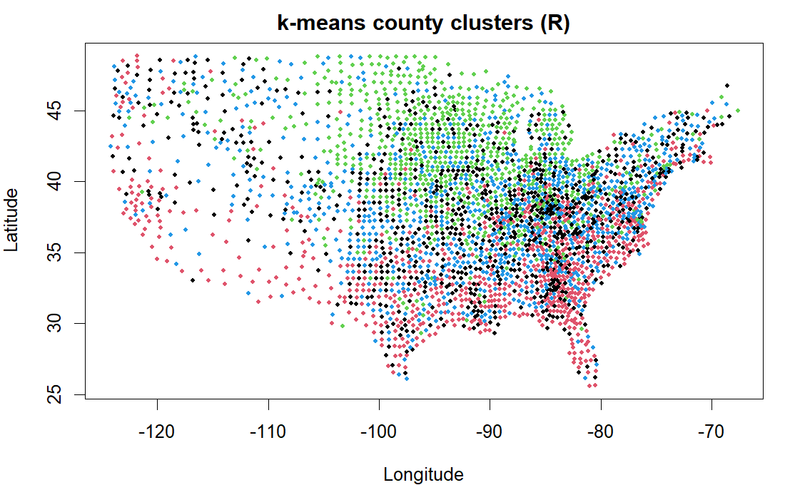
R output. Result:
cl 1 2 3 4 852 716 808 733# ACS counties: k-means clustering on socioeconomic profile, mapped by cluster. # counties.csv, one row per US county: median_income = median household income; poverty_pct = percent in poverty; bachelors_pct = percent with a bachelor degree; median_age = median age. import pandas as pd, matplotlib.pyplot as plt from sklearn.cluster import KMeans; from sklearn.preprocessing import scale acs = pd.read_csv("https://paulinadelmundomd.com/data/acs/counties.csv") acs = acs[(acs.lon>-125)&(acs.lon<-66)&(acs.lat>24)&(acs.lat<50)] X = scale(acs[["median_income","poverty_pct","bachelors_pct","median_age"]]) cl = KMeans(4, n_init=10, random_state=0).fit_predict(X) plt.scatter(acs.lon, acs.lat, c=cl, cmap="tab10", s=6); plt.title("k-means clusters (Python)") pd.Series(cl).value_counts().sort_index()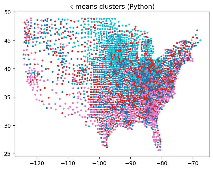
Python output. Result:
0 813 1 844 2 712 3 740 Name: count, dtype: int64 - K-nearest neighbours
-
A method that borrows from the k closest cases — the majority class for a label, or their average for a number, as when a missing value is filled from its nearest neighbours (imputation). Sensitive to scaling and to the choice of k. in the pathway →
Here it fills missing census-tract median income from geographic neighbours: hide 20% of Rhode Island’s tracts, impute each from the k = 10 nearest by location, and check the guess against the value we hid.
You can’t see the truth for a tract that is genuinely missing, so the error is judged by holding out known ones and comparing the guess to the value hidden. Across repeated hold-outs kNN is off by about 20%, versus 24% for filling every gap with the overall median — geography helps, but only modestly, since tract income is just somewhat spatially smooth. One split alone is optimistic and noisy, which is why the check is repeated; accuracy also hinges on k and on features sharing a scale, so the coordinates are converted to kilometres first.
# ACS Rhode Island census tracts: fill masked tract incomes from geographic neighbours. # ri_tracts.csv, one row per tract: lat/lon = tract centroid; median_income = median household income; poverty_pct, population. ri <- read.csv("https://paulinadelmundomd.com/data/acs/ri_tracts.csv") latkm <- ri$lat * 111.32 # a compact state: degrees -> km lonkm <- ri$lon * 111.32 * cos(mean(ri$lat) * pi / 180) k <- 10 impute <- function(tr, targets) # kNN regression: mean of the k nearest sapply(targets, function(i) { d <- sqrt((lonkm[tr]-lonkm[i])^2 + (latkm[tr]-latkm[i])^2) mean(ri$median_income[tr][order(d)[1:k]]) }) # assess by repeated hold-out: hide 20% of known tracts, impute, compare to truth err <- sapply(1:25, function(s) { set.seed(s) miss <- sample(nrow(ri), round(.2*nrow(ri))); tr <- setdiff(seq_len(nrow(ri)), miss) truth <- ri$median_income[miss] c(kNN = median(abs(impute(tr, miss)-truth)/truth)*100, baseline = median(abs(median(ri$median_income[tr])-truth)/truth)*100) }) # map one hold-out for illustration set.seed(1); miss <- sample(nrow(ri), round(.2*nrow(ri))); tr <- setdiff(seq_len(nrow(ri)), miss) imp <- ri$median_income; imp[miss] <- impute(tr, miss) col <- hcl.colors(100, "viridis")[cut(imp/1000, 100, labels = FALSE)] plot(ri$lon, ri$lat, col = col, pch = 16, cex = .8, xlab = "Longitude", ylab = "Latitude", main = "kNN imputation of tract median income - Rhode Island (R)") points(ri$lon[miss], ri$lat[miss], pch = 1, col = "#c02026", lwd = 1.3) # imputed round(rowMeans(err), 1) # median abs % error: kNN vs filling every gap with the median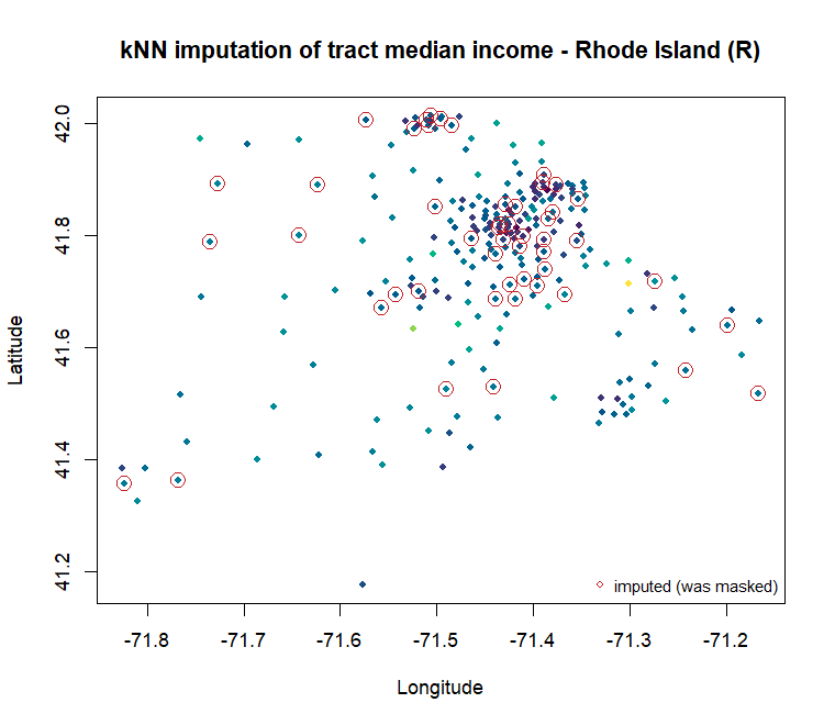
R output. Result:
kNN baseline 20.4 23.7# ACS Rhode Island census tracts: fill masked tract incomes from geographic neighbours. # ri_tracts.csv, one row per tract: lat/lon = tract centroid; median_income = median household income; poverty_pct, population. import numpy as np, pandas as pd, matplotlib.pyplot as plt from sklearn.impute import KNNImputer ri = pd.read_csv("https://paulinadelmundomd.com/data/acs/ri_tracts.csv") latkm = ri.lat * 111.32 # a compact state: degrees -> km lonkm = ri.lon * 111.32 * np.cos(np.radians(ri.lat.mean())) inc0 = ri.median_income.astype(float).values def holdout(seed): # hide 20%, impute, compare to truth rng = np.random.default_rng(seed) miss = rng.choice(len(ri), round(.2*len(ri)), replace=False) inc = inc0.copy(); truth = inc[miss].copy(); inc[miss] = np.nan filled = KNNImputer(n_neighbors=10).fit_transform(np.column_stack([lonkm, latkm, inc]))[:, 2] knn = np.median(np.abs(filled[miss]-truth)/truth) * 100 base = np.median(np.abs(np.nanmedian(inc)-truth)/truth) * 100 return miss, filled, knn, base # map one hold-out for illustration miss, filled, _, _ = holdout(1) plt.scatter(ri.lon, ri.lat, c=filled/1000, cmap="viridis", s=26) plt.scatter(ri.lon.values[miss], ri.lat.values[miss], s=60, facecolors="none", edgecolors="#c02026") plt.title("kNN imputation of tract median income - Rhode Island (Python)") # assess by repeated hold-out np.round(np.mean([holdout(s)[2:] for s in range(25)], axis=0), 1) # [kNN%, median-impute%]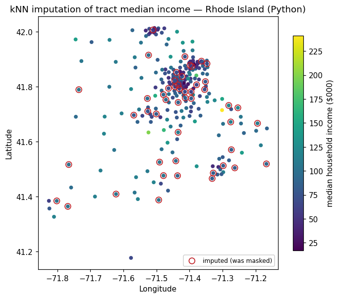
Python output. Result:
array([20.4, 23. ]) - Kaplan-Meier estimator
-
A nonparametric estimate of the survival curve from censored data, stepping down at each observed event and carrying censored subjects until they leave the risk set. in the pathway →
Median survival rises across arms, from 31.5 to 61.1 time units, with CIs quantifying each estimate. The curve reads as the probability of remaining event-free through each time point.
# CDISC ADaM ADTTE: Kaplan-Meier survival by arm (AVAL = time, event = 1 - CNSR). # adtte.csv, one row per subject, time-to-event: AVAL = time to event or censoring; CNSR = censoring flag, 1 = censored; TRTPN = treatment code. library(survival) adtte <- read.csv("https://paulinadelmundomd.com/data/cdisc/adtte.csv") km <- survfit(Surv(AVAL, 1 - CNSR) ~ TRTPN, data = adtte) plot(km, col = 1:3); print(km) # curves + median survival per arm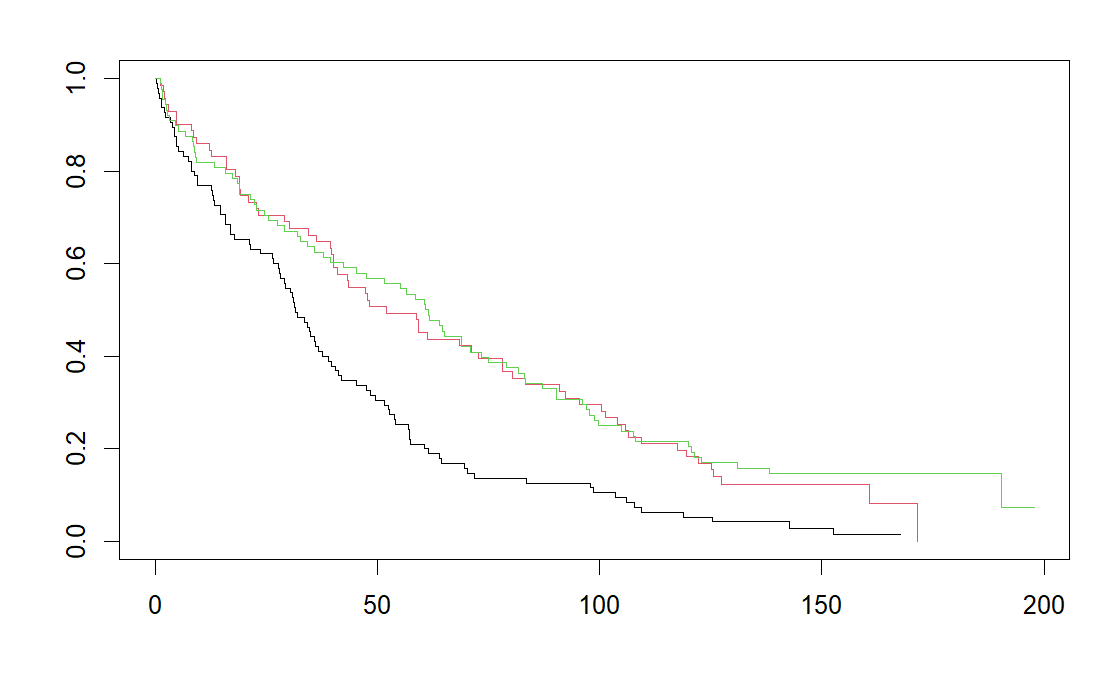
R output. Result:
Call: survfit(formula = Surv(AVAL, 1 - CNSR) ~ TRTPN, data = adtte) n events median 0.95LCL 0.95UCL TRTPN=0 95 93 31.5 27.8 39.6 TRTPN=54 71 64 52.1 40.2 78.2 TRTPN=81 88 76 61.1 42.3 79.0# CDISC ADaM ADTTE: Kaplan-Meier survival by arm (AVAL = time, event = 1 - CNSR). # adtte.csv, one row per subject, time-to-event: AVAL = time to event or censoring; CNSR = censoring flag, 1 = censored. import pandas as pd, matplotlib.pyplot as plt from lifelines import KaplanMeierFitter adtte = pd.read_csv("https://paulinadelmundomd.com/data/cdisc/adtte.csv"); adtte["event"] = 1 - adtte.CNSR for n, lab in [(0,"Placebo"), (54,"Low"), (81,"High")]: d = adtte[adtte.TRTPN == n] KaplanMeierFitter().fit(d.AVAL, d.event, label=lab).plot_survival_function(ci_show=False) plt.show()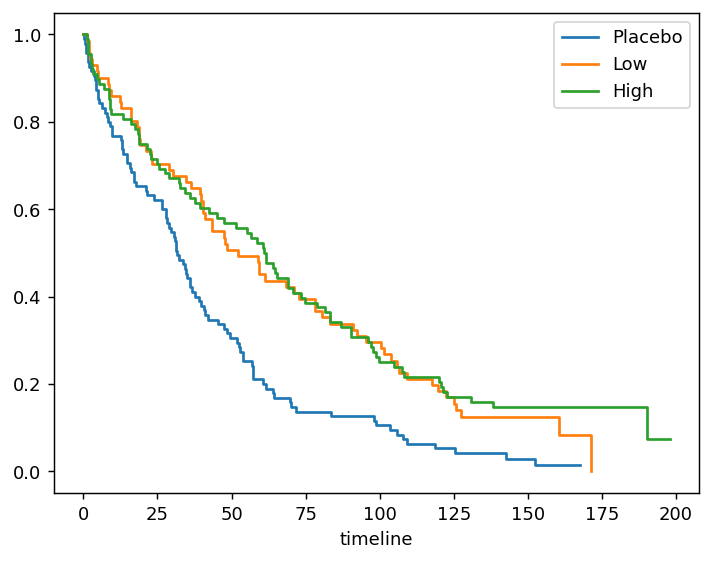
Python output. - Kendall’s tau
-
A measure of concordance between two ordinal rankings, with tau-c for rectangular tables. in the pathway →
\[\tau = \dfrac{C - D}{\binom{n}{2}}\]
where \(C\) and \(D\) count concordant and discordant pairs.
Tau of 0.73 means concordant pairs greatly outnumber discordant ones, a strong monotone association, and p is tiny. Tau is more conservative than Pearson and assumes no particular functional form.
# CDISC ADaM ADSL: correlation between baseline BMI and weight. # adsl.csv, one row per subject: BMIBL = baseline BMI; WEIGHTBL = baseline weight in kg. adsl <- read.csv("https://paulinadelmundomd.com/data/cdisc/adsl.csv") cor.test(adsl$BMIBL, adsl$WEIGHTBL, method = "kendall")Result:
Kendall's rank correlation tau data: adsl$BMIBL and adsl$WEIGHTBL z = 17.221, p-value < 2.2e-16 alternative hypothesis: true tau is not equal to 0 sample estimates: tau 0.7291097# CDISC ADaM ADSL: correlation between baseline BMI and weight. # adsl.csv, one row per subject. import pandas as pd; from scipy.stats import kendalltau adsl = pd.read_csv("https://paulinadelmundomd.com/data/cdisc/adsl.csv") kendalltau(adsl.BMIBL, adsl.WEIGHTBL)Result:
SignificanceResult(statistic=np.float64(0.7291096910754555), pvalue=np.float64(1.8319293482401593e-66)) - Kriging
- A geostatistical method for interpolating a continuous spatial surface (pollution, rainfall) from measurements at scattered points, predicting each unsampled location as a weighted average of observations. The weights come from a fitted semivariogram describing how similarity decays with distance, and kriging uniquely returns a prediction variance too, so uncertainty can be mapped alongside the estimate. It is the spatial analogue of best linear unbiased prediction. in the pathway → · Dohoo, Martin & Stryhn, 2012
- Kruskal-Wallis test
-
A rank-based alternative to one-way ANOVA when normality is doubtful. in the pathway →
\[H = \dfrac{12}{N(N+1)}\sum_{j}\dfrac{R_j^{2}}{n_j} - 3(N+1)\]
where \(R_j\) is the rank sum of group \(j\) of size \(n_j\), and \(N\) the total.
p below 0.001 means at least one arm’s change distribution sits systematically higher or lower than the others. It is the rank-based, non-normal analogue of one-way ANOVA.
# CDISC ADaM ADQS: rank-based test of Week-24 change across the three arms. # adqs.csv, one row per subject-visit: AVISIT = visit label; CHG = change from baseline; TRTP = treatment label. adqs <- read.csv("https://paulinadelmundomd.com/data/cdisc/adqs.csv"); wk24 <- subset(adqs, AVISIT == "Week 24") kruskal.test(CHG ~ TRTP, data = wk24)Result:
Kruskal-Wallis rank sum test data: CHG by TRTP Kruskal-Wallis chi-squared = 74.461, df = 2, p-value < 2.2e-16# CDISC ADaM ADQS: rank-based test of Week-24 change across the three arms. # adqs.csv, one row per subject-visit: AVISIT = visit label; TRTP = treatment label. import pandas as pd; from scipy.stats import kruskal wk24 = pd.read_csv("https://paulinadelmundomd.com/data/cdisc/adqs.csv").query("AVISIT == 'Week 24'") kruskal(*[g.CHG.values for _, g in wk24.groupby("TRTP")])Result:
KruskalResult(statistic=np.float64(74.46071492705049), pvalue=np.float64(6.777369974793549e-17)) - Kurtosis
-
A summary of a distribution’s tail-heaviness, part of reading its shape. in the pathway →
\[\gamma_2 = E\!\left[\left(\dfrac{X-\mu}{\sigma}\right)^{4}\right]\]
where higher kurtosis means heavier tails and more outliers; the normal distribution has \(\gamma_2 = 3\), so excess kurtosis is \(\gamma_2 - 3\).
Excess kurtosis near 0 (0.03) means median income has tails about as heavy as a normal distribution’s. Positive values flag fat tails (frequent extremes); it is read alongside skewness when judging whether a variable is safe to treat as normal.
# ACS counties: excess kurtosis of median income, a summary of tail-heaviness # (fourth central moment / variance^2, minus 3 so a normal reads 0). # counties.csv, one row per US county. cty <- read.csv("https://paulinadelmundomd.com/data/acs/counties.csv") x <- cty$median_income; m <- mean(x) mean((x - m)^4) / mean((x - m)^2)^2 - 3 # excess kurtosisResult:
[1] 0.03265697# ACS counties: excess kurtosis of median income, a summary of tail-heaviness # (fourth central moment / variance^2, minus 3 so a normal reads 0). # counties.csv, one row per US county. import pandas as pd, numpy as np cty = pd.read_csv("https://paulinadelmundomd.com/data/acs/counties.csv") x = cty.median_income.to_numpy(); m = x.mean() float(np.mean((x - m)**4) / np.mean((x - m)**2)**2 - 3) # excess kurtosisResult:
0.03265697370233367
L
- Landmark analysis
- A fix for immortal time bias: pick a fixed landmark time, classify each patient’s exposure status as of that moment, and start the clock there. Because follow-up begins at the landmark, the event-free waiting stretch is no longer wrongly credited to the exposed group. in the pathway →
- Lasso
-
L1 regularization that shrinks some coefficients exactly to zero and so also selects variables. in the pathway → · Tibshirani, 1996
\[\hat{\beta} = \operatorname*{arg\,min}_{\beta}\ \|Y - X\beta\|^2 + \lambda \sum_j |\beta_j|\]
where the L1 penalty \(\lambda \sum |\beta_j|\) shrinks coefficients and sets some exactly to zero, doing variable selection. To make R and Python solve the identical problem, predictors are standardized and a single \(\lambda\) is fixed (rather than cross-validated), with glmnet’s \(\lambda\) mapped to scikit-learn’s \(C = 1/(n\lambda)\).
With predictors standardized and lambda fixed, glmnet and scikit-learn now return the same coefficients. The L1 penalty keeps comorbidity (about +0.49) as the dominant predictor with small age and n_visits terms, and zeroes out sex and exposed entirely, which is the variable selection lasso is used for. Coefficients are on the standardized log-odds scale and shrunk toward zero, so treat the survivors as selected predictors rather than unbiased effects. In practice lambda would be cross-validated; it is fixed here only so the two languages line up.
# OMOP cohort: lasso (L1) logistic regression, standardized, fixed lambda. # cohort.csv, one row per person: age; sex (M/F); comorbidity; exposed 0/1; n_visits; outcome 0/1. library(glmnet) coh <- read.csv("https://paulinadelmundomd.com/data/omop/cohort.csv") X <- scale(model.matrix(outcome ~ age + sex + comorbidity + exposed + n_visits, coh)[, -1]) fit <- glmnet(X, coh$outcome, family = "binomial", alpha = 1, lambda = 0.02, standardize = FALSE) round(setNames(as.vector(coef(fit)), rownames(coef(fit))), 3) # named: intercept + 5 coefficientsResult:
(Intercept) age sexM comorbidity exposed n_visits -0.924 -0.054 0.000 0.490 0.000 -0.004# OMOP cohort: lasso (L1) logistic regression, standardized, fixed lambda. # cohort.csv, one row per person: age; sex (M/F); comorbidity; exposed 0/1; n_visits; outcome 0/1. import pandas as pd, numpy as np from sklearn.linear_model import LogisticRegression coh = pd.read_csv("https://paulinadelmundomd.com/data/omop/cohort.csv") X = pd.get_dummies(coh[["age", "sex", "comorbidity", "exposed", "n_visits"]], drop_first=True).astype(float) X = X[["age", "sex_M", "comorbidity", "exposed", "n_visits"]] # match R's column order Xs = (X - X.mean()) / X.std() # standardize like R's scale() lam = 0.02; C = 1 / (len(coh) * lam) # glmnet lambda -> sklearn C fit = LogisticRegression(penalty="l1", C=C, solver="saga", max_iter=500000, tol=1e-9).fit(Xs, coh.outcome) dict(zip(["(Intercept)"] + list(X.columns), np.round(np.r_[fit.intercept_, fit.coef_[0]], 3)))Result:
{'(Intercept)': np.float64(-0.924), 'age': np.float64(-0.054), 'sex_M': np.float64(0.0), 'comorbidity': np.float64(0.49), 'exposed': np.float64(0.0), 'n_visits': np.float64(-0.004)} - LATE
- The local average treatment effect, the contrast of potential outcomes among compliers. in the pathway → \[\mathrm{LATE} = \dfrac{\mathbb{E}[Y\mid Z=1]-\mathbb{E}[Y\mid Z=0]}{\mathbb{E}[A\mid Z=1]-\mathbb{E}[A\mid Z=0]}\] where the Wald ratio with instrument \(Z\) and treatment \(A\), identifying the effect among compliers.
- Latent class analysis
- A way to estimate the sensitivity and specificity of two or more tests, and the disease prevalence, when no gold standard exists, by treating true disease status as an unobserved (latent) variable inferred from the pattern of agreement across the tests. Its load-bearing assumption is that the tests err independently given true status; when they share a failure mode a conditional-dependence model is needed, and with only two tests the model is not identified without extra constraints. in the pathway → · Dohoo, Martin & Stryhn, 2012
- Lead-time bias
- The apparent survival gain from diagnosing earlier without changing the disease course. in the pathway →
- Leading question
- A survey item whose wording presses the respondent toward a particular answer. in the pathway → · Dohoo, Martin & Stryhn, 2012
- Learning algorithms and ensembles
- The supervised toolkit beyond regression, including k-nearest neighbours, support vector machines, decision trees, and ensembles. in the pathway →
- Leave-one-out and specification curves
- Re-estimating after dropping a single unit, or across many defensible modeling choices, to expose whether a finding rests on one unit or holds broadly. in the pathway →
- Left truncation
- Delayed entry: a subject is observed only from some time after the true origin, because they had to stay event-free long enough to be enrolled, as with prevalent cases or when age is the time scale. Unlike right censoring, which is missing follow-up at the end, left truncation hides the early at-risk period, and treating such data as if followed from the origin biases results in an immortal-time-like way. It is handled by entering each subject into the risk set only at their actual start time. in the pathway → · Dohoo, Martin & Stryhn, 2012
- Length-time bias
- The over-representation of slow, indolent cases that screening preferentially catches. in the pathway →
- Life table (actuarial method)
- The oldest survival method: event times are grouped into fixed intervals and the conditional probability of surviving each interval, given entry to it, is estimated and chained into a survival curve. Within an interval it assumes censored subjects are at risk for half the interval on average. The Kaplan-Meier estimator is its refinement, using exact event times rather than fixed intervals and so avoiding that approximation. in the pathway → · Dohoo, Martin & Stryhn, 2012
- Likelihood ratio test
-
A test comparing two nested models by twice the difference in their maximized log-likelihoods, referred to a chi-square with degrees of freedom equal to the parameter difference. in the pathway →
Adding treatment improves fit far beyond chance (deviance 38.7, p below 0.001), so the larger model is justified. The test compares nested models by how much the log-likelihood improves.
# LR test comparing nested logistic models (does treatment add fit?). # adqs.csv, one row per subject-visit: AVISIT = visit label; CHG = change from baseline; TRTPN = treatment code. adqs <- read.csv("https://paulinadelmundomd.com/data/cdisc/adqs.csv"); wk24 <- subset(adqs, AVISIT == "Week 24") wk24$resp <- as.integer(wk24$CHG <= -4) m0 <- glm(resp ~ AGE, wk24, family = binomial) m1 <- glm(resp ~ AGE + TRTPN, wk24, family = binomial) anova(m0, m1, test = "LRT")Result:
Analysis of Deviance Table Model 1: resp ~ AGE Model 2: resp ~ AGE + TRTPN Resid. Df Resid. Dev Df Deviance Pr(>Chi) 1 252 245.64 2 251 206.91 1 38.727 4.873e-10 *** --- Signif. codes: 0 '***' 0.001 '**' 0.01 '*' 0.05 '.' 0.1 ' ' 1# LR test comparing nested logistic models (does treatment add fit?). # adqs.csv, one row per subject-visit: AVISIT = visit label; TRTPN = treatment code. import pandas as pd, statsmodels.formula.api as smf; from scipy.stats import chi2 wk24 = pd.read_csv("https://paulinadelmundomd.com/data/cdisc/adqs.csv").query("AVISIT == 'Week 24'").assign(resp=lambda d: (d.CHG <= -4).astype(int)) m0 = smf.logit("resp ~ AGE", wk24).fit(disp=0) m1 = smf.logit("resp ~ AGE + TRTPN", wk24).fit(disp=0) chi2.sf(2 * (m1.llf - m0.llf), 1) # likelihood ratio test p-valueResult:
4.873225493946555e-10 - Likelihood ratios
-
Summaries of a diagnostic table independent of prevalence that update pre-test odds to post-test odds directly: \(LR^+ = Se/(1-Sp)\) and \(LR^- = (1-Se)/Sp\), with post-test odds \(=\) LR \(\times\) pre-test odds. An \(LR\) far from 1 moves the diagnosis; near 1 it barely helps. in the pathway → · Dohoo, Martin & Stryhn, 2012
\[\text{LR}+ = \frac{\text{sens}}{1 - \text{spec}}, \quad \text{LR}- = \frac{1 - \text{sens}}{\text{spec}}, \quad \text{post-test odds} = \text{pre-test odds} \times \text{LR}\]
where \(\text{LR}+\) is the positive likelihood ratio, how much a positive result raises the odds; \(\text{LR}-\) is the negative likelihood ratio, how much a negative result lowers the odds; \(\text{sens}\) is the sensitivity of the test; \(\text{spec}\) is the specificity of the test; \(\text{pre-test odds}\) is the odds of disease before the test, from prevalence; \(\text{post-test odds}\) is the odds of disease after the test result.
A positive test multiplies the pre-test odds by 1.7 and a negative test by 0.65. Both are modest; an LR+ above 10 or an LR- below 0.1 moves probability decisively.
# OMOP cohort: positive and negative likelihood ratios at a 0.3 threshold. # cohort.csv, one row per person: age = age in years; sex = sex (M/F); comorbidity = comorbidity count; exposed = drug exposure, 0/1; outcome = outcome condition, 0/1. coh <- read.csv("https://paulinadelmundomd.com/data/omop/cohort.csv") p <- predict(glm(outcome ~ age + sex + comorbidity + exposed, coh, family=binomial), type="response") pos <- p > 0.3 sens <- mean(pos[coh$outcome==1]); spec <- mean(!pos[coh$outcome==0]) c(LRpos = sens/(1-spec), LRneg = (1-sens)/spec)Result:
LRpos LRneg 1.7288862 0.6492807# OMOP cohort: positive and negative likelihood ratios at a 0.3 threshold. # cohort.csv, one row per person: age = age in years; sex = sex (M/F); comorbidity = comorbidity count; exposed = drug exposure, 0/1; outcome = outcome condition, 0/1. import pandas as pd, statsmodels.formula.api as smf coh = pd.read_csv("https://paulinadelmundomd.com/data/omop/cohort.csv") p = smf.logit("outcome ~ age + C(sex) + comorbidity + exposed", coh).fit(disp=0).predict() pos = p > 0.3; y = coh.outcome sens = pos[y==1].mean(); spec = (~pos[y==0]).mean() dict(LRpos=round(sens/(1-spec),2), LRneg=round((1-sens)/spec,2))Result:
{'LRpos': np.float64(1.73), 'LRneg': np.float64(0.65)} - Likert scale
- An ordinal rating scale on which the respondent marks their level of agreement (for example strongly agree, agree, neither, disagree, strongly disagree). Five to seven points are usual; an even number of points drops the neutral middle, giving a forced-choice scale. Treating the numbers as interval data and reporting means or SDs is only defensible with at least five points and roughly equal spacing. Items are often added into a summated scale. in the pathway → · Dohoo, Martin & Stryhn, 2012
- Linear combinations and contrasts
-
A weighted sum of regression coefficients reported as the quantity of interest, with a standard error drawn from the variance-covariance matrix. in the pathway →
\[L = c^{\top}\beta = \sum_j c_j \beta_j, \qquad \widehat{\operatorname{Var}}(L) = c^{\top}\widehat{\Sigma}\,c\]
where \(c\) is the vector of chosen weights, \(\beta\) the coefficients, and \(\widehat{\Sigma}\) their estimated variance-covariance matrix; its off-diagonal covariances are why the contrast’s standard error is not the individual coefficient standard errors combined.
The two oldest age bands differ by -0.008 in log-odds (SE 0.18), indistinguishable from zero. A contrast lets you estimate or test any linear combination of coefficients – a subgroup effect, a difference of differences – directly, with the correct standard error from the coefficient covariance.
# OMOP cohort: a contrast, a weighted sum of coefficients reported with its own # estimate and standard error. Here the difference between two age-band log-odds # from a logistic model, via L'b and sqrt(L' V L). cohort.csv: age, outcome. coh <- read.csv("https://paulinadelmundomd.com/data/omop/cohort.csv") coh$ageg <- cut(coh$age, c(0, 40, 55, 70, Inf)); m <- glm(outcome ~ ageg, binomial, coh) L <- c(0, 0, 1, -1) # (55,70] minus (70,Inf] c(sum(L * coef(m)), sqrt(as.numeric(t(L) %*% vcov(m) %*% L))) # estimate, SEResult:
[1] -0.008274483 0.181903216# OMOP cohort: a contrast, a weighted sum of coefficients reported with its own # estimate and standard error. Here the difference between two age-band log-odds # from a logistic model, via L'b and sqrt(L' V L). cohort.csv: age, outcome. import pandas as pd, numpy as np, statsmodels.formula.api as smf coh = pd.read_csv("https://paulinadelmundomd.com/data/omop/cohort.csv") coh["ageg"] = pd.cut(coh.age, [0, 40, 55, 70, np.inf]); m = smf.logit("outcome ~ C(ageg)", coh).fit(disp=0) L = np.array([0, 0, 1, -1.0]) # (55,70] minus (70,inf] np.array([L @ m.params.values, np.sqrt(L @ m.cov_params().values @ L)]) # estimate, SEResult:
array([-0.00827448, 0.18190327]) - Linear regression
-
A regression for continuous outcomes, returning a mean difference. in the pathway →
\[\hat\beta = \operatorname*{arg\,min}_{\beta}\,\lVert Y - X\beta\rVert^{2} \;\Rightarrow\; X^{\top}(Y - X\hat\beta) = 0 \;\Rightarrow\; \hat\beta = (X^{\top}X)^{-1} X^{\top} Y\]
where \(\beta\) are the coefficients (a mean difference per unit of each predictor) and \(E[Y \mid X] = X\beta\). Minimizing the squared residuals, then setting the derivative to zero, yields the normal equations \(X^{\top}(Y - X\hat\beta) = 0\), whose solution is the ordinary least squares estimate.
Each coefficient is the mean change in the outcome per one-unit rise in that predictor with the others held fixed; the dose slope here is about -0.05 units. The p-values say whether each is distinguishable from zero.
# CDISC ADaM ADQS: linear model of Week-24 change on treatment, age, sex. # adqs.csv, one row per subject-visit: AVISIT = visit label; CHG = change from baseline; TRTPN = treatment code. adqs <- read.csv("https://paulinadelmundomd.com/data/cdisc/adqs.csv"); wk24 <- subset(adqs, AVISIT == "Week 24") summary(lm(CHG ~ TRTPN + AGE + SEX, data = wk24))Result:
Call: lm(formula = CHG ~ TRTPN + AGE + SEX, data = wk24) Residuals: Min 1Q Median 3Q Max -9.6784 -1.9696 0.0677 2.1999 7.6708 Coefficients: Estimate Std. Error t value Pr(>|t|) (Intercept) -1.241479 2.043414 -0.608 0.544 TRTPN -0.051590 0.005416 -9.525 <2e-16 *** AGE 0.036665 0.026594 1.379 0.169 SEXM -0.232298 0.378883 -0.613 0.540 --- Signif. codes: 0 '***' 0.001 '**' 0.01 '*' 0.05 '.' 0.1 ' ' 1 Residual standard error: 2.998 on 250 degrees of freedom ... (truncated)# CDISC ADaM ADQS: linear model of Week-24 change on treatment, age, sex. # adqs.csv, one row per subject-visit: AVISIT = visit label; CHG = change from baseline; TRTPN = treatment code. import pandas as pd, statsmodels.formula.api as smf wk24 = pd.read_csv("https://paulinadelmundomd.com/data/cdisc/adqs.csv").query("AVISIT == 'Week 24'") smf.ols("CHG ~ TRTPN + AGE + SEX", data=wk24).fit().summary()Result:
OLS Regression Results ============================================================================== Dep. Variable: CHG R-squared: 0.282 Model: OLS Adj. R-squared: 0.273 Method: Least Squares F-statistic: 32.66 Prob (F-statistic): 7.55e-18 Log-Likelihood: -637.27 No. Observations: 254 AIC: 1283. Df Residuals: 250 BIC: 1297. Df Model: 3 Covariance Type: nonrobust ============================================================================== coef std err t P>|t| [0.025 0.975] ------------------------------------------------------------------------------ Intercept -1.2415 2.043 -0.608 0.544 -5.266 2.783 SEX[T.M] -0.2323 0.379 -0.613 0.540 -0.979 0.514 TRTPN -0.0516 0.005 -9.525 0.000 -0.062 -0.041 AGE 0.0367 0.027 1.379 0.169 -0.016 0.089 ... (truncated) - Link function
-
In a generalized linear model, the function that maps the mean of the outcome onto the linear predictor, so a possibly bounded mean is modeled on an unbounded linear scale; predictions come back through the inverse link, which keeps them in range. You choose it to match the outcome: the identity link for a continuous outcome (linear regression), the logit for a binary one (logistic regression, where coefficients are log odds ratios), and the log for counts or rates (Poisson regression, where coefficients are log rate ratios); the link paired naturally with a distribution is its canonical link. in the pathway →
\[g\big(E[Y \mid X]\big) = X\beta \;\Rightarrow\; E[Y \mid X] = g^{-1}(X\beta)\]
\[x_j \mapsto x_j + 1:\quad X\beta \mapsto X\beta + \beta_j, \qquad \mu \mapsto e^{\beta_j}\,\mu\]
where \(g\) is the link (identity \(g(\mu)=\mu\), logit \(g(\mu)=\ln\frac{\mu}{1-\mu}\), log \(g(\mu)=\ln\mu\)) and \(g^{-1}\) its inverse, which maps the linear predictor back into the mean’s range (for the logit, the sigmoid \(\mu = 1/(1+e^{-X\beta})\)). A one-unit rise in \(x_j\) adds \(\beta_j\) on the link scale; for a log-type link that multiplies the mean by \(e^{\beta_j}\), the factor read as an odds ratio (logit) or rate ratio (log), while for the identity link it is the additive mean difference \(\beta_j\).
The prevalence 0.29 is a log-odds of -0.89 on the logit scale. The link function lets a GLM keep a linear predictor while respecting the outcome’s range; its inverse (here the logistic function) maps predictions back to probabilities in [0, 1].
# OMOP cohort: the logit link of a generalized linear model maps a probability to # the log-odds scale on which the model is linear: g(p) = log(p / (1 - p)). Here # applied to the outcome prevalence. cohort.csv: outcome (0/1). coh <- read.csv("https://paulinadelmundomd.com/data/omop/cohort.csv") p <- mean(coh$outcome) log(p / (1 - p)) # logit (log-odds)Result:
[1] -0.8856903# OMOP cohort: the logit link of a generalized linear model maps a probability to # the log-odds scale on which the model is linear: g(p) = log(p / (1 - p)). Here # applied to the outcome prevalence. cohort.csv: outcome (0/1). import pandas as pd, numpy as np coh = pd.read_csv("https://paulinadelmundomd.com/data/omop/cohort.csv") p = coh.outcome.mean() float(np.log(p / (1 - p))) # logit (log-odds)Result:
-0.8856902914254381 - LOESS smoother
- A smoother drawn on a scatter to reveal the shape of a relationship before assuming it is linear. in the pathway →
- Log-binomial model
-
A generalized linear model for a binary outcome with a log link, so its coefficients exponentiate straight to a risk ratio or prevalence ratio rather than an odds ratio. It is the honest alternative to logistic regression when the outcome is common, though it can fail to converge, in which case a Poisson model with robust standard errors is the usual fallback. in the pathway → · Dohoo, Martin & Stryhn, 2012
The risk ratio is 0.84, read straight off exp(coef) because the log link models log-risk. Log-binomial gives the more interpretable risk ratio (an odds ratio overstates it when the outcome is common) but can fail to converge as fitted risks approach 1, where Poisson-with-robust-SE is the fallback.
# OMOP cohort: a log-binomial model -- a GLM for a binary outcome with a log # link, so exp(coef) is a risk ratio directly (not an odds ratio). # cohort.csv: outcome (0/1), exposed (0/1). coh <- read.csv("https://paulinadelmundomd.com/data/omop/cohort.csv") unname(exp(coef(glm(outcome ~ exposed, binomial(link = "log"), coh))["exposed"])) # risk ratioResult:
[1] 0.8447156# OMOP cohort: a log-binomial model -- a GLM for a binary outcome with a log # link, so exp(coef) is a risk ratio directly (not an odds ratio). # cohort.csv: outcome (0/1), exposed (0/1). import pandas as pd, numpy as np, statsmodels.api as sm, statsmodels.formula.api as smf coh = pd.read_csv("https://paulinadelmundomd.com/data/omop/cohort.csv") m = smf.glm("outcome ~ exposed", data=coh, family=sm.families.Binomial(link=sm.families.links.Log())).fit() float(np.exp(m.params["exposed"])) # risk ratioResult:
0.8447156320270875 - Log-rank test
-
A nonparametric test comparing survival curves. At each event time it computes how many events each group would show if survival were identical, subtracts that expected count from the observed, and sums the gaps across all times; a large total signals a real difference. It usually pairs with a Cox hazard ratio. in the pathway →
Chi-square 20.7 on 2 df (p < 0.001) means the survival curves differ across arms more than chance allows. The test compares whole curves but gives no effect size, so pair it with a hazard ratio.
# CDISC ADaM ADTTE: log-rank test comparing survival across arms. # adtte.csv, one row per subject, time-to-event: AVAL = time to event or censoring; CNSR = censoring flag, 1 = censored; TRTPN = treatment code. library(survival) adtte <- read.csv("https://paulinadelmundomd.com/data/cdisc/adtte.csv") survdiff(Surv(AVAL, 1 - CNSR) ~ TRTPN, data = adtte)Result:
Call: survdiff(formula = Surv(AVAL, 1 - CNSR) ~ TRTPN, data = adtte) N Observed Expected (O-E)^2/E (O-E)^2/V TRTPN=0 95 93 62.9 14.43 20.51 TRTPN=54 71 64 74.4 1.46 2.16 TRTPN=81 88 76 95.7 4.06 7.05 Chisq= 20.7 on 2 degrees of freedom, p= 3e-05# CDISC ADaM ADTTE: log-rank test comparing survival across arms. # adtte.csv, one row per subject, time-to-event. import pandas as pd; from lifelines.statistics import multivariate_logrank_test adtte = pd.read_csv("https://paulinadelmundomd.com/data/cdisc/adtte.csv") r = multivariate_logrank_test(adtte.AVAL, adtte.TRTPN, 1 - adtte.CNSR) r.test_statistic, r.p_value # chi-square statistic and p-valueResult:
(np.float64(20.71986180378755), np.float64(3.167664492112985e-05)) - Logistic regression
-
A regression for binary outcomes, returning an odds ratio. in the pathway →
\[\operatorname{logit}(p_i) = \ln\dfrac{p_i}{1-p_i} = X_i\beta \;\Rightarrow\; p_i = \frac{1}{1 + e^{-X_i\beta}}\]
\[\hat\beta = \operatorname*{arg\,max}_{\beta}\,\sum_i \big[\,y_i \ln p_i + (1-y_i)\ln(1-p_i)\,\big]\]
where \(p_i = P(Y_i=1 \mid X_i)\). The link maps the probability to a linear predictor; the Bernoulli log-likelihood has no closed-form maximum, so \(\hat\beta\) is found by iteratively reweighted least squares (Newton-Raphson). Each coefficient is a log odds ratio, so exponentiating gives the odds ratio.
Each dose unit multiplies the odds of the outcome by 1.038, about 3.8% higher, with a CI (1.02 to 1.05) that excludes 1. Odds ratios are not risk ratios and the two diverge when the outcome is common.
# CDISC ADaM: responder = ADAS-Cog improved by >= 4 points at Week 24. # adqs.csv, one row per subject-visit: AVISIT = visit label; CHG = change from baseline; TRTPN = treatment code. adqs <- read.csv("https://paulinadelmundomd.com/data/cdisc/adqs.csv") wk24 <- subset(adqs, AVISIT == "Week 24") wk24$responder <- as.integer(wk24$CHG <= -4) fit <- glm(responder ~ TRTPN + AGE, data = wk24, family = binomial) exp(cbind(OR = coef(fit), confint(fit))) # odds ratios + 95% CIResult:
OR 2.5 % 97.5 % (Intercept) 0.3357589 0.007757084 13.239110 TRTPN 1.0376281 1.023765596 1.054780 AGE 0.9681992 0.922611079 1.015391# CDISC ADaM: responder = ADAS-Cog improved by >= 4 points at Week 24. # adqs.csv, one row per subject-visit: TRTPN = treatment code. import numpy as np, pandas as pd, statsmodels.formula.api as smf adqs = pd.read_csv("https://paulinadelmundomd.com/data/cdisc/adqs.csv") wk24 = adqs[adqs.AVISIT == "Week 24"].copy() wk24["responder"] = (wk24.CHG <= -4).astype(int) fit = smf.logit("responder ~ TRTPN + AGE", data=wk24).fit() np.exp(fit.params) # odds ratiosResult:
Optimization terminated successfully. Current function value: 0.407311 Iterations 7 Intercept 0.335759 TRTPN 1.037628 AGE 0.968199 dtype: float64 - Log-likelihood
-
The logarithm of the likelihood, turning the product over independent observations into a sum that is far easier to differentiate and maximize; its maximizer is the maximum likelihood estimate. in the pathway →
\[\ell(\theta) = \log L(\theta) = \sum_i \log f(y_i;\theta)\]
where \(f(y_i;\theta)\) is the model’s density for observation \(y_i\).
The maximized log-likelihood is -565 (higher, i.e. less negative, is better). Taking the log turns the product over independent observations into a sum, which is why fitting maximizes the log-likelihood; -2 times it is the deviance.
# OMOP cohort: the log-likelihood of a fitted logistic model -- the log of the # probability of the observed outcomes under the fit, what maximum likelihood # maximizes and what deviance, AIC, and the LR test are built on. # cohort.csv: outcome, age, comorbidity. coh <- read.csv("https://paulinadelmundomd.com/data/omop/cohort.csv") as.numeric(logLik(glm(outcome ~ age + comorbidity, binomial, coh))) # log-likelihoodResult:
[1] -564.9856# OMOP cohort: the log-likelihood of a fitted logistic model -- the log of the # probability of the observed outcomes under the fit, what maximum likelihood # maximizes and what deviance, AIC, and the LR test are built on. # cohort.csv: outcome, age, comorbidity. import pandas as pd, statsmodels.formula.api as smf coh = pd.read_csv("https://paulinadelmundomd.com/data/omop/cohort.csv") float(smf.logit("outcome ~ age + comorbidity", coh).fit(disp=0).llf) # log-likelihoodResult:
-564.9855842298268 - Log-logistic distribution
- A survival distribution giving a single-peaked hazard that rises then falls, useful when risk first climbs then eases. It serves as a parametric baseline in accelerated failure time models, which describe treatment as speeding up or slowing down the time to an event. in the pathway →
- Log-normal distribution
-
A distribution for a positive quantity whose logarithm is normal, so it is right-skewed with a long tail. As a survival baseline it also gives a hazard that rises then falls, used in accelerated failure time models (which describe treatment as speeding up or slowing down time to an event). in the pathway →
The geometric mean income is $56,406, below the arithmetic mean because the distribution is right-skewed. For a log-normal variable the geometric mean estimates the median, and analyses often model log(x) so the symmetric, constant-variance normal assumptions apply.
# ACS counties: the geometric mean of median income, exp(mean(log(x))), the # natural center for a right-skewed, log-normal quantity (one whose logarithm is # normal). counties.csv, one row per US county. cty <- read.csv("https://paulinadelmundomd.com/data/acs/counties.csv") exp(mean(log(cty$median_income))) # geometric meanResult:
[1] 56405.69# ACS counties: the geometric mean of median income, exp(mean(log(x))), the # natural center for a right-skewed, log-normal quantity (one whose logarithm is # normal). counties.csv, one row per US county. import pandas as pd, numpy as np cty = pd.read_csv("https://paulinadelmundomd.com/data/acs/counties.csv") float(np.exp(np.log(cty.median_income).mean())) # geometric meanResult:
56405.69262605992 - Log odds (logit)
-
The natural log of the odds, the linear predictor of logistic regression; a logistic coefficient is a difference in log odds, that is a log odds ratio, so it is 0 when there is no effect (an odds ratio of 1) and exponentiating it returns the odds ratio. The log scale is symmetric and additive, so a doubling and a halving of the odds sit equal and opposite distances from 0, which is why a confidence interval for any ratio measure is computed on the log scale and then exponentiated. in the pathway →
\[\operatorname{logit}(p) = \ln\dfrac{p}{1-p}, \qquad \beta = \ln(\mathrm{OR})\]
where \(p\) is the event probability, \(p/(1-p)\) the odds, and \(\beta\) a logistic coefficient (a log odds ratio).
The empirical log-odds (logit) of the proportion is -0.016; exponentiating returns the odds of any adverse event, about 0.98 – near even, since about half of subjects have one. Log-odds are the additive scale logistic regression works on, where a coefficient is a difference of log-odds (a log odds ratio) and the sign alone gives direction.
# CDISC ADaM: log odds (logit) of having any adverse event. # adsl.csv, one row per subject: USUBJID = subject id linking the tables. # adae.csv, one row per adverse-event record. adsl <- read.csv("https://paulinadelmundomd.com/data/cdisc/adsl.csv"); adae <- read.csv("https://paulinadelmundomd.com/data/cdisc/adae.csv") p <- mean(adsl$USUBJID %in% adae$USUBJID) log(p / (1 - p)) # log odds; qlogis(p) is identicalResult:
[1] -0.01574836# CDISC ADaM: log odds (logit) of having any adverse event. # adsl.csv, one row per subject. # adae.csv, one row per adverse-event record. import pandas as pd; from scipy.special import logit adsl = pd.read_csv("https://paulinadelmundomd.com/data/cdisc/adsl.csv"); adae = pd.read_csv("https://paulinadelmundomd.com/data/cdisc/adae.csv") p = adsl.USUBJID.isin(adae.USUBJID).mean() logit(p) # log odds (= log(p / (1 - p)))Result:
-0.01574835696813914 - LOINC lab codes
- Logical Observation Identifiers Names and Codes, a standard vocabulary for identifying laboratory tests and clinical observations. in the pathway → · Regenstrief: LOINC ↗
- Lookback window
- The pre-index period in which confounders are measured so adjustment targets baseline causes, not post-exposure variables. in the pathway →
M
- MAD
-
The median absolute deviation: take each point’s distance from the median, then take the median of those distances. A spread measure that resists outliers; it is often rescaled by 1.4826 so it matches the standard deviation under a normal. in the pathway →
\[\text{MAD} = \operatorname{median}\big(|x_i - \operatorname{median}(x)|\big)\]
where the median of the absolute deviations from the median; a robust spread measure far less sensitive to outliers than the standard deviation.
The MAD is $6,090: half the counties sit within that distance of the median. Because it uses medians throughout, one extreme county cannot inflate it, which makes MAD (often scaled by 1.4826 to match a normal’s SD) the robust alternative to the standard deviation.
# ACS counties: the median absolute deviation of median income, a robust spread # measure -- the median distance of each value from the overall median, unmoved # by the outliers that inflate a standard deviation. counties.csv. cty <- read.csv("https://paulinadelmundomd.com/data/acs/counties.csv") x <- cty$median_income median(abs(x - median(x))) # median absolute deviationResult:
[1] 6090# ACS counties: the median absolute deviation of median income, a robust spread # measure -- the median distance of each value from the overall median, unmoved # by the outliers that inflate a standard deviation. counties.csv. import pandas as pd, numpy as np cty = pd.read_csv("https://paulinadelmundomd.com/data/acs/counties.csv") x = cty.median_income.to_numpy() float(np.median(np.abs(x - np.median(x)))) # median absolute deviationResult:
6090.0 - Mann-Whitney test
-
A rank-based alternative to the two-group t-test when normality is doubtful, also called the Wilcoxon rank-sum. in the pathway →
\[U = R_1 - \dfrac{n_1(n_1+1)}{2}\]
where \(R_1\) is the rank sum of group 1 of size \(n_1\).
p < 0.001 means one arm’s change values tend to rank above the other’s. It tests a shift between distributions using ranks, so it does not require normal data, and R’s W and Python’s U are the same statistic (7172) once the groups are given in the same order.
# CDISC ADaM ADQS: Mann-Whitney U on Week-24 change, high dose vs placebo. # adqs.csv, one row per subject-visit: AVISIT = visit label; CHG = change from baseline; TRTP = treatment label. adqs <- read.csv("https://paulinadelmundomd.com/data/cdisc/adqs.csv") wk24 <- subset(adqs, AVISIT == "Week 24" & TRTP %in% c("Placebo","Xanomeline High Dose")) wilcox.test(CHG ~ TRTP, data = wk24)Result:
Wilcoxon rank sum test with continuity correction data: CHG by TRTP W = 7172, p-value < 2.2e-16 alternative hypothesis: true location shift is not equal to 0# CDISC ADaM ADQS: Mann-Whitney U on Week-24 change, high dose vs placebo. # adqs.csv, one row per subject-visit: AVISIT = visit label. import pandas as pd; from scipy.stats import mannwhitneyu wk24 = pd.read_csv("https://paulinadelmundomd.com/data/cdisc/adqs.csv").query("AVISIT == 'Week 24'") pl, hi = (wk24.CHG[wk24.TRTP == t] for t in ["Placebo", "Xanomeline High Dose"]) mannwhitneyu(pl, hi) # U for Placebo, matching R's WResult:
MannwhitneyuResult(statistic=np.float64(7172.0), pvalue=np.float64(6.488094244780918e-17)) - Mantel-Haenszel estimator
-
A method for pooling stratum-specific odds ratios, risk ratios, or rate ratios into one. in the pathway → · Dohoo, Martin & Stryhn, 2012
\[\widehat{\text{OR}}_{\text{MH}} = \dfrac{\sum_k a_k d_k / n_k}{\sum_k b_k c_k / n_k}\]
where \(a_k, b_k, c_k, d_k\) are the 2x2 cell counts in stratum \(k\) with total \(n_k\); it pools stratum-specific association while adjusting for the stratifying confounder.
Pooling across sex strata, the common odds ratio stays above 1 with p=0.002, so the association holds after stratifying. Mantel-Haenszel assumes the stratum-specific effect is roughly constant.
# CDISC ADaM: Mantel-Haenszel OR of an AE by arm, stratified by sex. # adsl.csv, one row per subject: USUBJID = subject id linking the tables; TRT01PN = arm code, 0 = placebo; SEX = sex (M/F). # adae.csv, one row per adverse-event record: AEDECOD = adverse-event term. adsl <- read.csv("https://paulinadelmundomd.com/data/cdisc/adsl.csv"); adae <- read.csv("https://paulinadelmundomd.com/data/cdisc/adae.csv") adsl$dz <- as.integer(adsl$USUBJID %in% adae$USUBJID[adae$AEDECOD=="DIZZINESS"]) mantelhaen.test(table(adsl$TRT01PN > 0, adsl$dz, adsl$SEX))Result:
Mantel-Haenszel chi-squared test with continuity correction data: table(adsl$TRT01PN > 0, adsl$dz, adsl$SEX) Mantel-Haenszel X-squared = 9.8734, df = 1, p-value = 0.001677 alternative hypothesis: true common odds ratio is not equal to 1 95 percent confidence interval: 1.763406 12.527136 sample estimates: common odds ratio 4.700045# CDISC ADaM: Mantel-Haenszel OR of an AE by arm, stratified by sex. # adsl.csv, one row per subject: SEX = sex (M/F). # adae.csv, one row per adverse-event record. import pandas as pd; from statsmodels.stats.contingency_tables import StratifiedTable adsl = pd.read_csv("https://paulinadelmundomd.com/data/cdisc/adsl.csv"); adae = pd.read_csv("https://paulinadelmundomd.com/data/cdisc/adae.csv") adsl["dz"] = adsl.USUBJID.isin(adae.USUBJID[adae.AEDECOD=="DIZZINESS"]).astype(int) tabs = [pd.crosstab(g.TRT01PN > 0, g.dz).values for _, g in adsl.groupby("SEX")] StratifiedTable(tabs).oddsratio_pooled # Mantel-Haenszel pooled ORResult:
4.700045447659446 - MAR
- Missing at random: missingness depending only on observed data, handled by multiple imputation conditional on it. in the pathway →
- Marginal likelihood
- The probability the model assigns to the observed data, averaged over all parameter values weighted by the prior. It is the normalizing constant in Bayes’ theorem (also called the evidence) and is what Bayesian model comparison weighs. in the pathway → \[p(x) = \int p(x \mid \theta)\,p(\theta)\,d\theta\] where \(p(\theta)\) is the prior and \(p(x\mid\theta)\) the likelihood.
- Marginal model
- A model for clustered data that estimates the population-average effect of a covariate, averaged over clusters, rather than its effect within a given cluster. It contrasts with a conditional, subject-specific model such as a random-effects mixed model, whose coefficients hold a cluster’s random effect fixed. For a linear model the two coincide, but under a nonlinear link such as logistic the population-average odds ratio is pulled toward the null relative to the subject-specific one, so they answer different questions. GEE fits marginal models directly. in the pathway → · Dohoo, Martin & Stryhn, 2012
- Marginal structural model
-
A model for the treatment effect that first reweights patients to break the tangle between past treatment and evolving confounders, then estimates the effect on the balanced pseudo-population (a g-method, fitted by inverse-probability-of-treatment weighting). in the pathway → · Robins et al., 2000
\[sw_i = \prod_t \dfrac{P(A_t \mid \bar A_{t-1})}{P(A_t \mid \bar A_{t-1},\, \bar L_t)}\]
where each subject is weighted by \(sw_i\), the product over time of the marginal probability of the observed treatment over its probability given the covariate history \(\bar L_t\). Dividing by the latter breaks the confounder-treatment link, building a pseudo-population in which a simple weighted regression of the outcome on treatment \(A_t\) recovers the causal effect; the numerator stabilizes the weights to tame their variance.
In the IPTW-weighted model the exposure lowers the log-odds by 0.25 (p=0.012), the causal contrast in the pseudo-population. MSMs handle time-varying confounding that ordinary adjustment mishandles.
# OMOP cohort: MSM - IPTW-weighted outcome model (marginal exposure effect). # cohort.csv, one row per person: age = age in years; sex = sex (M/F); comorbidity = comorbidity count; exposed = drug exposure, 0/1; outcome = outcome condition, 0/1. coh <- read.csv("https://paulinadelmundomd.com/data/omop/cohort.csv") ps <- predict(glm(exposed ~ age + sex + comorbidity, data = coh, family = binomial), type="response") w <- ifelse(coh$exposed==1, 1/ps, 1/(1-ps)) summary(glm(outcome ~ exposed, data = coh, family = binomial, weights = w))$coefficientsResult:
Estimate Std. Error z value Pr(>|z|) (Intercept) -0.7615181 0.06698423 -11.368617 5.992945e-30 exposed -0.2503869 0.10005237 -2.502558 1.232994e-02# OMOP cohort: MSM - IPTW-weighted outcome model (marginal exposure effect). # cohort.csv, one row per person: age = age in years; sex = sex (M/F); comorbidity = comorbidity count; exposed = drug exposure, 0/1; outcome = outcome condition, 0/1. import numpy as np, pandas as pd, statsmodels.formula.api as smf, statsmodels.api as sm coh = pd.read_csv("https://paulinadelmundomd.com/data/omop/cohort.csv") ps = smf.logit("exposed ~ age + C(sex) + comorbidity", coh).fit(disp=0).predict() coh["w"] = np.where(coh.exposed==1, 1/ps, 1/(1-ps)) smf.glm("outcome ~ exposed", coh, family=sm.families.Binomial(), freq_weights=coh.w).fit().paramsResult:
Intercept -0.761518 exposed -0.250387 dtype: float64 - Markov chain Monte Carlo (MCMC)
- A family of algorithms that fit Bayesian models by drawing a dependent sequence of samples whose stationary distribution is the posterior, used when the posterior has no closed form. Gibbs sampling and Metropolis-Hastings are the workhorses; the early draws before the chain settles (the burn-in) are discarded, and convergence is checked with trace plots, multiple chains, and the \(\hat{R}\) statistic. Because successive draws are correlated, the effective sample size is smaller than the number of iterations. in the pathway → · Dohoo, Martin & Stryhn, 2012
- Markov model
-
A state-transition model moving a cohort between health states each cycle by a transition matrix, the standard tool for chronic disease. in the pathway →
\[p = 1 - \exp(-r \cdot t)\]
where \(p\) is the per-cycle transition probability; \(r\) is the rate reported in the published evidence; \(t\) is the cycle length over which the probability applies.
After ten cycles the 1000-person cohort has moved to about 107 healthy, 269 sick, and 624 dead. The trace shows how a fixed transition matrix carries a cohort through states over time.
# Three-state Markov cohort (Healthy, Sick, Dead) traced over 10 cycles. P <- matrix(c(.80,.15,.05, 0,.85,.15, 0,0,1), 3, byrow=TRUE) state <- c(1000, 0, 0) for (i in 1:10) state <- state %*% P round(state, 1) # cohort distribution after 10 cyclesResult:
[,1] [,2] [,3] [1,] 107.4 268.5 624.1# Three-state Markov cohort (Healthy, Sick, Dead) traced over 10 cycles. import numpy as np P = np.array([[.80,.15,.05],[0,.85,.15],[0,0,1]]); state = np.array([1000.,0,0]) for _ in range(10): state = state @ P state.round(1) # cohort distribution after 10 cyclesResult:
[107.4 268.5 624.1] - Matching
- Choosing comparison subjects to share the confounders’ distribution with the index group, breaking the confounder-exposure link by design. In a cohort study it makes exposed and unexposed alike on the matched factors; in a case-control study it does not by itself remove confounding but forces a matched analysis that does. Variants include pair, frequency (category-level), and caliper matching. Matching on a factor forfeits studying that factor’s own effect and risks overmatching when the factor lies on the causal path. in the pathway → · Dohoo, Martin & Stryhn, 2012
- Maximum likelihood estimation (MLE)
-
The default way a regression’s coefficients are fit: choose the parameter values that make the observed data most probable under the model, with large-sample standard errors read off the curvature of the log-likelihood. It is the estimation engine beneath the GLM and most of the regression families. in the pathway →
\[L(\theta) = \prod_{i} f(y_i;\theta) \;\Rightarrow\; \ell(\theta) = \sum_{i} \log f(y_i;\theta) \;\Rightarrow\; \left.\frac{\partial \ell}{\partial \theta}\right|_{\hat\theta} = 0\]
\[\widehat{\operatorname{Var}}(\hat\theta) = I(\hat\theta)^{-1}, \qquad I(\theta) = -\,\frac{\partial^{2} \ell}{\partial \theta\,\partial \theta^{\top}}\]
where \(L\) is the likelihood (the joint probability of the data read as a function of \(\theta\)), \(\ell\) its logarithm, and \(f(y_i;\theta)\) the model’s density for observation \(y_i\). Setting the score \(\partial\ell/\partial\theta\) to zero and solving gives the estimate \(\hat\theta\) (in closed form for some models, by iteration for most); the observed information \(I\), the curvature of \(\ell\) at \(\hat\theta\), inverts to the large-sample variance.
The MLE standard deviation is 15.97 (dividing by n); the usual unbiased estimate divides by n-1 and is slightly larger. Maximum likelihood – the parameter values that make the observed data most probable – is how nearly every regression coefficient in this glossary is fit.
# OMOP cohort: the maximum-likelihood estimate of a normal's standard deviation # divides by n (not n-1), since MLE maximizes the data's probability without the # unbiasedness correction. cohort.csv: age. coh <- read.csv("https://paulinadelmundomd.com/data/omop/cohort.csv") a <- coh$age sqrt(mean((a - mean(a))^2)) # MLE of the SD (divides by n)Result:
[1] 15.97242# OMOP cohort: the maximum-likelihood estimate of a normal's standard deviation # divides by n (not n-1), since MLE maximizes the data's probability without the # unbiasedness correction. cohort.csv: age. import pandas as pd, numpy as np coh = pd.read_csv("https://paulinadelmundomd.com/data/omop/cohort.csv") a = coh.age.to_numpy() float(np.sqrt(np.mean((a - a.mean())**2))) # MLE of the SD (divides by n)Result:
15.972422608984523 - Maximum tolerated dose
- The highest tolerable dose, the target a phase I dose-finding study estimates. in the pathway →
- MCAR
- Missing completely at random: a benign mechanism where missingness is unrelated to any data. in the pathway →
- McFadden’s pseudo-R-squared
-
A rough stand-in for R-squared in generalized linear models, where a true R-squared does not apply. Higher means the predictors add more over a no-predictor model, but it is not on a 0-to-1 scale: values of 0.2 to 0.4 already indicate a good fit. in the pathway →
\[R^{2}_{\text{McF}} = 1 - \dfrac{\ln \hat L_{\text{full}}}{\ln \hat L_{\text{null}}}\]
where \(\hat L\) are the fitted and intercept-only model likelihoods.
McFadden’s pseudo R-squared is 0.064. Its scale is not the proportion of variance explained (0.2-0.4 already signals a good fit), so it is read differently from an ordinary R-squared and mainly used to compare models on the same data.
# OMOP cohort: McFadden's pseudo R-squared for a logistic model, 1 minus the # ratio of the fitted to the null (intercept-only) log-likelihood -- a rough # stand-in where a true R-squared does not exist. cohort.csv: outcome, age, comorbidity. coh <- read.csv("https://paulinadelmundomd.com/data/omop/cohort.csv") m <- glm(outcome ~ age + comorbidity, binomial, coh) 1 - as.numeric(logLik(m)) / as.numeric(logLik(glm(outcome ~ 1, binomial, coh))) # McFadden R2Result:
[1] 0.06448924# OMOP cohort: McFadden's pseudo R-squared for a logistic model, 1 minus the # ratio of the fitted to the null (intercept-only) log-likelihood -- a rough # stand-in where a true R-squared does not exist. cohort.csv: outcome, age, comorbidity. import pandas as pd, statsmodels.formula.api as smf coh = pd.read_csv("https://paulinadelmundomd.com/data/omop/cohort.csv") m = smf.logit("outcome ~ age + comorbidity", coh).fit(disp=0) float(1 - m.llf / m.llnull) # McFadden R2Result:
0.06448924343110451 - MCMC
- Markov chain Monte Carlo: drawing a dependent sequence of samples whose long-run distribution is the posterior. in the pathway →
- McNemar’s test
-
A test of whether two paired dichotomous measurements (the same subjects assessed two ways) call positives at different rates, built only from the discordant pairs: \(\chi^2 = (n_{12} - n_{21})^2/(n_{12} + n_{21})\). A significant result means one test yields more positives than the other, so assessing their agreement may be beside the point. in the pathway → · Dohoo, Martin & Stryhn, 2012
The statistic 6.43 (chi-square, 1 df, p about 0.01) says the two measurements disagree asymmetrically. McNemar discards the concordant pairs entirely – agreement carries no information about change – which makes it the right test for paired binary data, unlike an ordinary chi-square.
# McNemar's test for two paired dichotomous measurements (the same subjects # assessed twice): the chi-square uses only the discordant pairs, (b - c)^2 / # (b + c). Here 25 changed one way and 10 the other. b <- 25; c <- 10 (b - c)^2 / (b + c) # McNemar chi-squareResult:
[1] 6.428571# McNemar's test for two paired dichotomous measurements (the same subjects # assessed twice): the chi-square uses only the discordant pairs, (b - c)^2 / # (b + c). Here 25 changed one way and 10 the other. b, c = 25, 10 (b - c)**2 / (b + c) # McNemar chi-squareResult:
6.428571428571429 - Mean absolute error
-
A prediction error measure in the outcome’s units, used when a few large errors should not dominate. in the pathway →
\[\mathrm{MAE} = \dfrac{1}{n}\sum_{i=1}^{n}\lvert y_i - \hat y_i\rvert\]
where \(y_i\) is the observed and \(\hat y_i\) the predicted value across \(n\) cases.
Predictions miss by about $3,543 on average. MAE reports error in the outcome’s units and weights every miss equally, so it is more robust and more interpretable than RMSE, which squares errors and penalizes the occasional large miss far more heavily.
# ACS counties: mean absolute error of a linear model's predictions, the average # size of the residuals in the outcome's own units -- less swayed by a few large # errors than the squared-error RMSE. counties.csv. cty <- read.csv("https://paulinadelmundomd.com/data/acs/counties.csv") mean(abs(resid(lm(median_income ~ poverty_pct + bachelors_pct, cty)))) # MAEResult:
[1] 3543.075# ACS counties: mean absolute error of a linear model's predictions, the average # size of the residuals in the outcome's own units -- less swayed by a few large # errors than the squared-error RMSE. counties.csv. import pandas as pd, statsmodels.formula.api as smf cty = pd.read_csv("https://paulinadelmundomd.com/data/acs/counties.csv") float(smf.ols("median_income ~ poverty_pct + bachelors_pct", cty).fit().resid.abs().mean()) # MAEResult:
3543.075172792336 - Measurement error and misclassification
- Imprecision in measuring a variable, whose effect on an estimate depends on whether the error relates to the outcome. in the pathway → · Dohoo, Martin & Stryhn, 2012
- Measurement-method effects
- Two devices or protocols measuring the same quantity can disagree systematically, so a threshold validated under one does not transfer. in the pathway →
- Measures of disease frequency
- The standard forms for counting how often disease occurs, including prevalence, incidence, and rates. in the pathway → \[\text{prevalence}=\dfrac{\text{cases}}{N},\qquad \text{incidence rate}=\dfrac{\text{new cases}}{\text{person-time}}\]
- Mediation analysis
-
Splitting a total effect into a direct effect and an indirect effect running through a mediator. in the pathway →
\[\text{total} = \text{direct} + \text{indirect}, \quad \text{indirect} = a \cdot b\]
where \(\text{total}\) is the total effect of the exposure on the outcome; \(\text{direct}\) is the effect not running through the mediator; \(\text{indirect}\) is the effect running through the mediator; \(a\) is the exposure-to-mediator coefficient; \(b\) is the mediator-to-outcome coefficient.
About -666 dollars per poverty-point of poverty’s association with income runs through education. The product a*b splits a total effect into direct and indirect paths; it rests on strong no-unmeasured-confounding assumptions for both the exposure and the mediator, where mediation analysis is most often criticized.
# ACS counties: a mediation analysis by the product method. The indirect effect # of poverty on income through education is a*b: a = poverty's effect on the # mediator (bachelors_pct), b = the mediator's effect on income given poverty. cty <- read.csv("https://paulinadelmundomd.com/data/acs/counties.csv") a <- coef(lm(bachelors_pct ~ poverty_pct, cty))["poverty_pct"] b <- coef(lm(median_income ~ bachelors_pct + poverty_pct, cty))["bachelors_pct"] unname(a * b) # indirect (mediated) effectResult:
[1] -665.9171# ACS counties: a mediation analysis by the product method. The indirect effect # of poverty on income through education is a*b: a = poverty's effect on the # mediator (bachelors_pct), b = the mediator's effect on income given poverty. import pandas as pd, statsmodels.formula.api as smf cty = pd.read_csv("https://paulinadelmundomd.com/data/acs/counties.csv") a = smf.ols("bachelors_pct ~ poverty_pct", cty).fit().params["poverty_pct"] b = smf.ols("median_income ~ bachelors_pct + poverty_pct", cty).fit().params["bachelors_pct"] float(a * b) # indirect (mediated) effectResult:
-665.917051266747 - Mediator
- A variable on the causal path from exposure to outcome, left alone when the total effect is the target. in the pathway → · Dohoo, Martin & Stryhn, 2012
- Medication administration record (MAR)
- The inpatient log of doses actually given to a patient, the closest data source to a drug truly taken, as opposed to an order written or a prescription merely dispensed. in the pathway →
- Medication possession ratio (MPR)
- Total days supplied divided by days in the observation interval, an adherence measure that can exceed one with overlaps. in the pathway → \[\text{MPR} = \dfrac{\text{days supplied}}{\text{days in the period}}\] where days supplied is summed over fills in the measurement period; MPR can exceed 1 when fills overlap, which is why PDC is often preferred.
- Meta-analysis
-
The statistical combination of results from multiple studies into a single pooled estimate more precise than any one study. Each study’s effect is weighted, usually by the inverse of its variance, and combined under a fixed-effect model (one true effect) or a random-effects model (the true effect varies across studies). It is only as sound as the systematic review that assembled the inputs; heterogeneity and publication bias are the standing threats. in the pathway → · Dohoo, Martin & Stryhn, 2012
The random-effects pool gives a log-odds of about -0.29 (95% CI -0.43 to -0.14), a real protective effect, while I-squared near 71% flags substantial between-study heterogeneity. Report the pooled effect with both its CI and this heterogeneity; the wide prediction interval (a separate entry) is the more honest summary of what a new study might show.
# Study-level meta-analysis (yi = log OR, sei = SE): random-effects pool + forest plot. # studies.csv, one row per trial in a meta-analysis: study = study label; yi = effect estimate, log odds ratio; sei = standard error of yi. library(metafor) d <- read.csv("https://paulinadelmundomd.com/data/meta/studies.csv") res <- rma(yi = yi, sei = sei, data = d, method = "DL") # random-effects (DerSimonian-Laird) forest(res, slab = d$study) res # pooled log-OR, CI, tau^2, I^2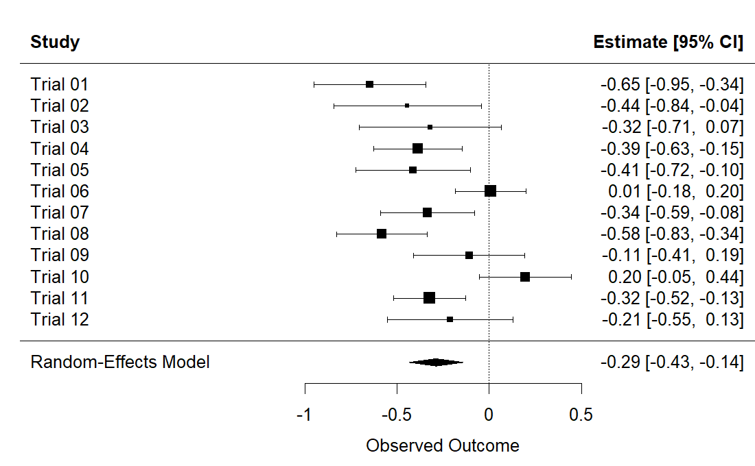
R output. Result:
Random-Effects Model (k = 12; tau^2 estimator: DL) tau^2 (estimated amount of total heterogeneity): 0.0449 (SE = 0.0282) tau (square root of estimated tau^2 value): 0.2119 I^2 (total heterogeneity / total variability): 70.90% H^2 (total variability / sampling variability): 3.44 Test for Heterogeneity: Q(df = 11) = 37.8039, p-val < .0001 Model Results: estimate se zval pval ci.lb ci.ub -0.2880 0.0740 -3.8921 <.0001 -0.4330 -0.1430 *** --- Signif. codes: 0 '***' 0.001 '**' 0.01 '*' 0.05 '.' 0.1 ' ' 1# studies.csv, one row per trial in a meta-analysis: yi = effect estimate, log odds ratio. import numpy as np, pandas as pd d = pd.read_csv("https://paulinadelmundomd.com/data/meta/studies.csv") yi = d.yi.values; vi = d.sei.values**2; k = len(yi); w = 1/vi Q = (w*(yi - (w*yi).sum()/w.sum())**2).sum() tau2 = max(0, (Q-(k-1)) / (w.sum() - (w**2).sum()/w.sum())) wr = 1/(vi+tau2); mu = (wr*yi).sum()/wr.sum(); se = wr.sum()**-0.5 print("pooled logOR %.3f (95%% CI %.3f, %.3f); tau2=%.3f" % (mu, mu-1.96*se, mu+1.96*se, tau2))Result:
pooled logOR -0.288 (95% CI -0.433, -0.143); tau2=0.045 - Meta-regression
-
A technique that tries to explain heterogeneity across studies using study-level covariates. in the pathway →
Regressing the effect on publication year gives a slope of about 0.029 per year with p = 0.21, so year does not explain the between-study heterogeneity here. Meta-regression is observational across studies, so even a significant moderator would be associational rather than causal, and with only 12 studies it is low-powered.
# Inverse-variance weighted meta-regression of effect on publication year. # studies.csv, one row per trial: yi = effect (log OR); sei = SE of yi; year = publication year. d <- read.csv("https://paulinadelmundomd.com/data/meta/studies.csv") coef(summary(lm(yi ~ year, weights = 1/sei^2, data = d))) # estimate, SE, t, pResult:
Estimate Std. Error t value Pr(>|t|) (Intercept) -59.3507980 44.3677423 -1.337702 0.2106197 year 0.0293656 0.0220508 1.331725 0.2125075# Inverse-variance weighted meta-regression of effect on publication year. # studies.csv, one row per trial: yi = effect (log OR); sei = SE of yi; year = publication year. import pandas as pd, statsmodels.api as sm d = pd.read_csv("https://paulinadelmundomd.com/data/meta/studies.csv") w = 1/d.sei.values**2 sm.WLS(d.yi, sm.add_constant(d.year), weights=w).fit().summary2().tables[1]Result:
Coef. Std.Err. t P>|t| [0.025 0.975] const -59.350798 44.367742 -1.337702 0.210620 -158.208288 39.506692 year 0.029366 0.022051 1.331725 0.212507 -0.019767 0.078498 - Metropolis-Hastings
- An MCMC algorithm that proposes a move from the current values and accepts or rejects it with a probability set by the posterior ratio, so the chain visits each region in proportion to its posterior mass. It needs the posterior only up to a constant, which is why it works when direct sampling is impossible. in the pathway → \[p(\theta)\,q(\theta'\mid\theta)\,\alpha(\theta\to\theta') = p(\theta')\,q(\theta\mid\theta')\,\alpha(\theta'\to\theta) \;\Rightarrow\; \alpha = \min\!\left(1,\ \dfrac{p(\theta')\,q(\theta \mid \theta')}{p(\theta)\,q(\theta' \mid \theta)}\right)\] where \(q\) is the proposal density. Imposing detailed balance (reversibility with respect to the target \(p\)) on the move \(\theta\to\theta'\) forces the acceptance probability \(\alpha\); the target need only be known up to its normalizing constant, which cancels in the ratio.
- Micro-costing
- Bottom-up costing that counts each resource used and multiplies it by its unit price. in the pathway →
- Minimal clinically important difference
-
The smallest change in an outcome that patients or clinicians would regard as worthwhile, used to set the effect a study is powered to detect so that statistical significance tracks clinical importance rather than sample size. in the pathway →
The half-SD rule gives an MCID of about 8 units. Distribution-based MCIDs are convenient but arbitrary; anchor-based versions, tied to what patients report as a meaningful change, are preferred when available. The MCID is the yardstick a trial’s effect size must clear to matter clinically.
# A distribution-based minimal clinically important difference: a common # anchor-free rule takes half a standard deviation of the outcome as the smallest # change patients tend to notice. Here half the SD of age. cohort.csv: age. coh <- read.csv("https://paulinadelmundomd.com/data/omop/cohort.csv") 0.5 * sd(coh$age) # 0.5-SD distribution-based MCIDResult:
[1] 7.990207# A distribution-based minimal clinically important difference: a common # anchor-free rule takes half a standard deviation of the outcome as the smallest # change patients tend to notice. Here half the SD of age. cohort.csv: age. import pandas as pd coh = pd.read_csv("https://paulinadelmundomd.com/data/omop/cohort.csv") float(0.5 * coh.age.std(ddof=1)) # 0.5-SD distribution-based MCIDResult:
7.990207407471624 - Minimization
- An adaptive assignment that places each patient to keep arms balanced across several factors at once. in the pathway → · Pocock & Simon, 1975
- Minimum detectable effect
-
The smallest true effect a fixed sample can detect at a chosen power and significance level, obtained by solving the power relation for the effect instead of for the sample size. It answers what a size-constrained study can credibly find. in the pathway →
\[\mathrm{MDE} = (z_{1-\alpha/2}+z_{1-\beta})\,\sigma\sqrt{\tfrac{1}{n_1}+\tfrac{1}{n_2}}\]
where the power relation solved for the effect at fixed sample sizes \(n_1, n_2\).
With n=64 per group at 80% power, the smallest detectable standardized effect is about 0.5, a medium effect. Anything smaller than this would likely be missed by this design.
# Smallest effect size detectable with n=64/group at 80% power. library(pwr) pwr.t.test(n = 64, power = 0.8, sig.level = 0.05)$dResult:
[1] 0.499072# Smallest effect size detectable with n=64/group at 80% power. from statsmodels.stats.power import TTestIndPower TTestIndPower().solve_power(nobs1=64, power=0.8, alpha=0.05)Result:
0.4990691771904248 - Missing data
- Why a value is missing decides what can be done about it, across the MCAR, MAR, and MNAR mechanisms. in the pathway →
- Missing value code
- A dedicated code (for example -999) reserved for a missing answer, so a non-response is never confused with a real zero or with a value lost in data entry; dichotomous items are coded 0/1 consistently throughout. Getting this right at capture is what makes principled missing-data handling possible later. in the pathway → · Dohoo, Martin & Stryhn, 2012
- Mixed-effects models
-
Regression models that add random effects, cluster- or subject-specific deviations drawn from a distribution, to the usual fixed effects, so correlated or repeated measurements within a group are modeled rather than wrongly assumed independent. They are the likelihood-based, subject-specific counterpart to GEE, with MMRM the common continuous-outcome version for repeated measures over time. in the pathway →
\[Y_{ij} = X_{ij}\beta + Z_{ij} b_i + \varepsilon_{ij}, \qquad b_i \sim N(0, G)\]
where \(Y_{ij}\) is the \(j\)-th measurement on subject or cluster \(i\), \(X_{ij}\beta\) the fixed-effect (population-average) part, \(Z_{ij} b_i\) the random effects with subject-specific deviations \(b_i\) drawn from a mean-zero distribution of covariance \(G\), and \(\varepsilon_{ij}\) the residual error.
The random-intercept SD of 8.3 dwarfs the residual 2.6, so most variation is between subjects, which justifies the per-subject random effect. Fixed effects give the average trend; random effects capture individual departures.
# CDISC ADaM ADQS: random intercept per subject for repeated measures. # adqs.csv, one row per subject-visit: USUBJID = subject id; AVISITN = visit number; AVAL = score at that visit; TRTPN = treatment code. library(lme4) adqs <- read.csv("https://paulinadelmundomd.com/data/cdisc/adqs.csv") lmer(AVAL ~ AVISITN * TRTPN + (1 | USUBJID), data = adqs)Result:
Linear mixed model fit by REML ['lmerMod'] Formula: AVAL ~ AVISITN * TRTPN + (1 | USUBJID) Data: adqs REML criterion at convergence: 5810.153 Random effects: Groups Name Std.Dev. USUBJID (Intercept) 8.325 Residual 2.620 Number of obs: 1016, groups: USUBJID, 254 Fixed Effects: (Intercept) AVISITN TRTPN AVISITN:TRTPN 24.438911 0.062501 0.011567 -0.002162# CDISC ADaM ADQS: random intercept per subject for repeated measures. # adqs.csv, one row per subject-visit: USUBJID = subject id; AVISITN = visit number; AVAL = score at that visit; TRTPN = treatment code. import pandas as pd, statsmodels.formula.api as smf adqs = pd.read_csv("https://paulinadelmundomd.com/data/cdisc/adqs.csv") smf.mixedlm("AVAL ~ AVISITN * TRTPN", data=adqs, groups="USUBJID").fit().summary()Result:
Mixed Linear Model Regression Results ======================================================== Model: MixedLM Dependent Variable: AVAL No. Observations: 1016 Method: REML No. Groups: 254 Scale: 6.8634 Min. group size: 4 Log-Likelihood: -2905.0763 Max. group size: 4 Converged: Yes Mean group size: 4.0 -------------------------------------------------------- Coef. Std.Err. z P>|z| [0.025 0.975] -------------------------------------------------------- Intercept 24.439 0.857 28.502 0.000 22.758 26.119 AVISITN 0.063 0.015 4.285 0.000 0.034 0.091 TRTPN 0.012 0.015 0.750 0.453 -0.019 0.042 AVISITN:TRTPN -0.002 0.000 -8.236 0.000 -0.003 -0.002 USUBJID Var 69.309 2.787 ======================================================== - MMRM
- The mixed model for repeated measures, standard for a longitudinal trial endpoint, using all timepoints and handling dropout under missing-at-random. in the pathway →
- MNAR
- Missing not at random: missingness depending on the unseen value itself, needing pattern-mixture or tipping-point sensitivity approaches. in the pathway →
- Model fit, comparison, and prediction error
- The continuous-outcome counterpart to calibration and discrimination, covering variance explained, model comparison, and honest out-of-sample error. in the pathway →
- Model modifications
- Standard adaptations to a base regression, including splines, interactions, transformations, and offsets, each answering a specific signal. in the pathway →
- Model validation and calibration
- Checks that build trust in a model: verification that it is coded correctly, plus validation that it matches reality across face (does it look sensible to experts), internal (does it reproduce its own inputs), external (does it match independent data), and predictive (does it forecast future events) layers. in the pathway →
- Monte Carlo simulation
- Generating data under a known process and running the planned analysis over many replicates to study an estimator’s bias, coverage, and required sample size. in the pathway →
- Mortality rate
- The incidence rate of death: deaths from all causes per unit of person-time in a population. Strictly a rate, though the term is often loosely stretched to mean a risk of death, so read it with care. in the pathway → · Dohoo, Martin & Stryhn, 2012
- Multi-criteria decision analysis (MCDA)
- Explicitly weighting criteria such as equity and severity when a single ratio cannot capture value. in the pathway →
- Multinomial logistic regression
- A regression for an unordered categorical outcome with three or more levels, fitting a separate set of log-odds coefficients for each category against a common baseline, so it returns an odds ratio per predictor for every non-reference category. Unlike the proportional-odds model it assumes no ordering among the categories, which is what makes it the right choice when the levels are genuinely nominal. in the pathway →
- Multiple control groups
- Using two or more distinct control series, usually to hedge against a bias suspected in any single group. The return is generally small: if the groups agree on exposure a shared bias could still sit in both, and if they disagree there is seldom a principled basis for choosing between them, while the analysis only grows more complex. The common verdict is that a second control group adds little. in the pathway → · Dohoo, Martin & Stryhn, 2012
- Multiple imputation
- Filling in missing values conditional on observed data, valid when data are missing at random. in the pathway → · Rubin, 1976
- Multiplicity control
- Methods to rein in false positives when many hypotheses are tested, via family-wise error or false-discovery control. in the pathway →
- Multistage sampling
- Nesting sampling stages: sampling primary sampling units, then units within them, often with probability proportional to size. Cost-optimal allocation samples \(n_i=\sqrt{\frac{\sigma_i^2}{\sigma_g^2}\cdot\frac{c_g}{c_i}}\) units per group, trading between- and within-group variance against sampling costs. in the pathway → · Dohoo, Martin & Stryhn, 2012
- Mutually exclusive and exhaustive
- The two conditions for a sound set of response categories: no case fits more than one option (mutually exclusive) and every case fits some option (jointly exhaustive), the latter often secured by an ‘Other’ category. The same pair of requirements applies to any categorical variable. in the pathway → · Dohoo, Martin & Stryhn, 2012
N
- Naive Bayes
-
A classifier applying Bayes’ theorem under the simplifying assumption that features are independent given the class; fast and often competitive despite the unrealistic assumption. in the pathway →
The classifier is right about 69% of the time on the training data it was fit to (in-sample accuracy, which flatters the model). It assumes features are independent given the class, which is rarely exactly true but often works well enough.
# OMOP cohort: naive Bayes classifier for the outcome. # cohort.csv, one row per person: age = age in years; sex = sex (M/F); comorbidity = comorbidity count; exposed = drug exposure, 0/1; outcome = outcome condition, 0/1. library(e1071) coh <- read.csv("https://paulinadelmundomd.com/data/omop/cohort.csv") nb <- naiveBayes(factor(outcome) ~ age + sex + comorbidity + exposed, coh) mean(predict(nb, coh) == coh$outcome) # training accuracyResult:
[1] 0.685# OMOP cohort: naive Bayes classifier for the outcome. # cohort.csv, one row per person: age = age in years; sex = sex (M/F); comorbidity = comorbidity count; exposed = drug exposure, 0/1; outcome = outcome condition, 0/1. import pandas as pd; from sklearn.naive_bayes import GaussianNB coh = pd.read_csv("https://paulinadelmundomd.com/data/omop/cohort.csv") X = pd.get_dummies(coh[["age","sex","comorbidity","exposed"]], drop_first=True) nb = GaussianNB().fit(X, coh.outcome); (nb.predict(X) == coh.outcome).mean()Result:
0.685 - Natural direct and indirect effects
- The counterfactual framing of mediation, needing no unmeasured confounding of the mediator-outcome relationship. in the pathway → · Robins & Greenland, 1992
- NDC (National Drug Code)
- Identifier encoding drug manufacturer, product, and package, requiring mapping to reach the ingredient level. in the pathway → · FDA: National Drug Code Directory ↗
- Necessary cause
- A cause that must be present or the outcome simply cannot occur. In the sufficient-component framing, it is a component that appears in every sufficient cause. Few exposures for chronic disease are necessary; an infectious agent for its specific disease is the classic example. in the pathway → · Dohoo, Martin & Stryhn, 2012
- Negative binomial distribution
-
A distribution for overdispersed counts whose variance exceeds the mean. in the pathway →
\[\text{Var}(Y) = \mu + \dfrac{\mu^{2}}{\theta}\]
where \(\mu\) is the mean count and \(\theta\) the dispersion parameter; the variance exceeds the mean (overdispersion) and approaches the Poisson as \(\theta \to \infty\).
Here the ratio is 0.93, close to 1, so these visit counts are near-Poisson (a Poisson forces variance to equal the mean). When the ratio climbs well above 1 – common in utilization data with a few heavy users – the negative binomial’s extra dispersion parameter is what keeps the standard errors honest.
# OMOP cohort: the variance-to-mean ratio of a count, the diagnostic for # overdispersion. Above 1, counts are more variable than a Poisson allows and the # negative binomial (which adds a dispersion parameter) fits better. # cohort.csv: n_visits (a count). coh <- read.csv("https://paulinadelmundomd.com/data/omop/cohort.csv") var(coh$n_visits) / mean(coh$n_visits) # variance / meanResult:
[1] 0.9348351# OMOP cohort: the variance-to-mean ratio of a count, the diagnostic for # overdispersion. Above 1, counts are more variable than a Poisson allows and the # negative binomial (which adds a dispersion parameter) fits better. # cohort.csv: n_visits (a count). import pandas as pd coh = pd.read_csv("https://paulinadelmundomd.com/data/omop/cohort.csv") float(coh.n_visits.var(ddof=1) / coh.n_visits.mean()) # variance / meanResult:
0.934835120020305 - Negative binomial regression
-
A count regression used when overdispersion makes the variance exceed the mean. in the pathway →
\[\ln(\mu) = X\beta, \qquad \text{Var}(Y) = \mu + \dfrac{\mu^2}{\theta}\]
where like Poisson regression but with a dispersion parameter \(\theta\) that lets the variance exceed the mean, the usual situation with real counts.
exp(0.017) is about 1.02, so each dose unit raises the expected AE count by roughly 2%. Negative binomial is preferred over Poisson when counts are overdispersed, as its extra variance parameter allows here.
# CDISC ADaM: same AE count, allowing overdispersion (negative binomial). # adsl.csv, one row per subject: USUBJID = subject id linking the tables; TRT01PN = arm code, 0 = placebo. # adae.csv, one row per adverse-event record. library(MASS) adsl <- read.csv("https://paulinadelmundomd.com/data/cdisc/adsl.csv"); adae <- read.csv("https://paulinadelmundomd.com/data/cdisc/adae.csv") adsl$n_ae <- as.integer(table(factor(adae$USUBJID, levels = adsl$USUBJID))) glm.nb(n_ae ~ TRT01PN, data = adsl)Result:
Call: glm.nb(formula = n_ae ~ TRT01PN, data = adsl, init.theta = 1.113133121, link = log) Coefficients: (Intercept) TRT01PN -0.7386 0.0166 Degrees of Freedom: 253 Total (i.e. Null); 252 Residual Null Deviance: 285.9 Residual Deviance: 248.3 AIC: 717.8# CDISC ADaM: same AE count, allowing overdispersion (negative binomial). # adsl.csv, one row per subject: TRT01PN = arm code, 0 = placebo. # adae.csv, one row per adverse-event record. import pandas as pd, statsmodels.formula.api as smf adsl = pd.read_csv("https://paulinadelmundomd.com/data/cdisc/adsl.csv"); adae = pd.read_csv("https://paulinadelmundomd.com/data/cdisc/adae.csv") adsl["n_ae"] = adsl.USUBJID.map(adae.USUBJID.value_counts()).fillna(0) smf.negativebinomial("n_ae ~ TRT01PN", data=adsl).fit().summary()Result:
Optimization terminated successfully. Current function value: 1.401173 Iterations: 11 Function evaluations: 17 Gradient evaluations: 17 NegativeBinomial Regression Results ============================================================================== Dep. Variable: n_ae No. Observations: 254 Model: NegativeBinomial Df Residuals: 252 Method: MLE Df Model: 1 Pseudo R-squ.: 0.04649 Log-Likelihood: -355.90 converged: True LL-Null: -373.25 Covariance Type: nonrobust LLR p-value: 3.840e-09 ============================================================================== coef std err z P>|z| [0.025 0.975] ------------------------------------------------------------------------------ Intercept -0.7386 0.172 -4.306 0.000 -1.075 -0.402 ... (truncated) - Negative control exposure
-
An exposure sharing the real exposure’s confounding structure but with no plausible causal link to the outcome. in the pathway →
The permuted control shows a near-zero coefficient (0.20) with p=0.17, as a valid negative control should. A large or significant effect here would flag residual confounding or a bug in the pipeline, not a real association.
# A negative-control exposure should have no real effect on the outcome. # Build one by permuting the real exposure, then run the same adjusted model: # a coefficient far from zero would flag residual confounding in the pipeline. # cohort.csv, one row per person: age = age in years; sex = sex (M/F); comorbidity = comorbidity count; exposed = drug exposure, 0/1; outcome = outcome condition, 0/1. coh <- read.csv("https://paulinadelmundomd.com/data/omop/cohort.csv"); set.seed(4) coh$nc <- sample(coh$exposed) # permuted -> no association by construction m <- glm(outcome ~ nc + age + sex + comorbidity, data = coh, family = binomial) round(coef(summary(m))["nc", c("Estimate", "Pr(>|z|)")], 3)Result:
Estimate Pr(>|z|) 0.202 0.165# A negative-control exposure should have no real effect on the outcome. # Build one by permuting the real exposure, then run the same adjusted model: # a coefficient far from zero would flag residual confounding in the pipeline. # cohort.csv, one row per person: age = age in years; sex = sex (M/F); comorbidity = comorbidity count; exposed = drug exposure, 0/1; outcome = outcome condition, 0/1. import pandas as pd, numpy as np, statsmodels.formula.api as smf coh = pd.read_csv("https://paulinadelmundomd.com/data/omop/cohort.csv"); rng = np.random.default_rng(4) coh["nc"] = rng.permutation(coh["exposed"].values) # no association by construction m = smf.logit("outcome ~ nc + age + C(sex) + comorbidity", coh).fit(disp=0) round(m.params["nc"], 3), round(m.pvalues["nc"], 3)Result:
(np.float64(-0.234), np.float64(0.107)) - Negative control outcome
- An outcome sharing the real outcome’s confounding structure but that exposure cannot plausibly cause. in the pathway →
- Negative controls and calibration
- Using outcomes or exposures with known null effects to detect and correct residual confounding in real analyses. in the pathway →
- Nested case-control study
- A case-control study drawn from a source population that is fully enumerable, such as an existing cohort or registry, so the sampling fractions of both cases and controls are known. That is what lets it do the one thing ordinary case-control designs cannot: recover the disease frequency by exposure, because the outcome-dependent sampling is no longer anonymous. Because cases and controls come from the same base by construction it forecloses much selection bias, and it is the efficient way to assay costly stored biospecimens on a sampled subset rather than the whole cohort. in the pathway → · Dohoo, Martin & Stryhn, 2012
- Net benefit
-
A metric weighing true positives against false positives at a threshold probability, going beyond accuracy by accounting for the consequences of acting. in the pathway →
\[\mathrm{NB} = \dfrac{TP}{n} - \dfrac{FP}{n}\cdot\dfrac{p_t}{1-p_t}\]
where \(p_t\) is the threshold probability of acting and \(n\) the sample size.
Net benefit of 0.07 at a 30% threshold means using the model to decide is worth 0.07 net true-positive classifications per patient after each false positive is docked by the threshold odds. A decision curve plots this across thresholds against treat-all and treat-none, turning discrimination into clinical value.
# OMOP cohort: net benefit at a decision threshold, TP/n - FP/n * (pt/(1-pt)), # weighing true positives against false positives by the odds of the threshold # probability pt = 0.3. The basis of a decision curve. cohort.csv. coh <- read.csv("https://paulinadelmundomd.com/data/omop/cohort.csv") p <- predict(glm(outcome ~ age + comorbidity + n_visits, binomial, coh), type = "response") y <- coh$outcome; n <- length(y); pt <- 0.3; pred <- p >= pt sum(pred & y == 1)/n - sum(pred & y == 0)/n * (pt / (1 - pt)) # net benefitResult:
[1] 0.07014286# OMOP cohort: net benefit at a decision threshold, TP/n - FP/n * (pt/(1-pt)), # weighing true positives against false positives by the odds of the threshold # probability pt = 0.3. The basis of a decision curve. cohort.csv. import pandas as pd, numpy as np, statsmodels.formula.api as smf coh = pd.read_csv("https://paulinadelmundomd.com/data/omop/cohort.csv") p = np.asarray(smf.logit("outcome ~ age + comorbidity + n_visits", coh).fit(disp=0).predict()) y = coh.outcome.to_numpy(); n = len(y); pt = 0.3; pred = p >= pt float((pred & (y == 1)).sum()/n - (pred & (y == 0)).sum()/n * (pt / (1 - pt))) # net benefitResult:
0.07014285714285715 - Net monetary benefit
-
A restatement of a cost-effectiveness comparison as effect times willingness-to-pay minus cost. Because it is a difference rather than a ratio, it stays well-behaved when one option is both cheaper and better, a case where the ICER ratio breaks down. in the pathway →
\[\text{NMB} = \lambda \times E - C\]
where \(E\) is the health effect (QALYs), \(C\) the cost, and \(\lambda\) the willingness-to-pay threshold; a positive NMB means the option is cost-effective at \(\lambda\), and the highest-NMB option wins.
At a $50,000 willingness-to-pay threshold the strategy’s NMB is +$262,000, so its health gains outweigh its costs at that threshold. NMB flips sign as the threshold changes, so always state the threshold.
# Net monetary benefit at a willingness-to-pay threshold. qalys <- 6.2; cost <- 48000; wtp <- 50000 qalys * wtp - cost # NMB > 0 means cost-effective at this thresholdResult:
[1] 262000# Net monetary benefit at a willingness-to-pay threshold. qalys, cost, wtp = 6.2, 48000, 50000 qalys * wtp - cost # NMB > 0 means cost-effective at this thresholdResult:
262000.0 - Net reclassification index
- A measure of how much adding a predictor correctly reshuffles patients across risk categories: it rewards moving true cases into higher-risk bins and true non-cases into lower-risk bins. Sensitive to where the category cutoffs are drawn. in the pathway →
- Net-benefit regression
- Collapsing each patient’s cost and effect into a single net-benefit number at a willingness-to-pay threshold, then running an ordinary regression of it on treatment arm. Because it is now one continuous outcome, you can add covariates the usual way to adjust for imbalance. in the pathway → \[\mathrm{NMB}_i = \lambda E_i - C_i = \beta_0 + \beta_1\,\text{arm}_i + \varepsilon_i\] where \(\lambda\) is the willingness-to-pay threshold and \(\beta_1\) the incremental net benefit.
- Network meta-analysis
- Combining a whole network of trials to estimate every pairwise treatment contrast and rank options, even when no trial compared them all directly. in the pathway → \[\hat{d}_{AB} = \hat{d}_{AC} - \hat{d}_{BC}, \qquad \operatorname{Var}(\hat{d}_{AB}) = \operatorname{Var}(\hat{d}_{AC}) + \operatorname{Var}(\hat{d}_{BC})\] where \(\hat{d}_{XY}\) is the estimated contrast between treatments \(X\) and \(Y\) and \(C\) a common comparator; this Bucher indirect estimate adds the two variances, so it is less precise than a direct head-to-head, and a full network model pools direct and indirect evidence for every pair.
- Neural network
-
A model of stacked layers of weighted sums passed through nonlinear activations, fit by gradient descent; flexible but data-hungry and hard to interpret. in the pathway →
The network classifies the training cases correctly about 71% of the time (in-sample accuracy, so optimistic). On small tabular data it rarely beats simpler models, and it needs scaled inputs and careful tuning.
# OMOP cohort: single-hidden-layer neural network for the outcome. # cohort.csv, one row per person: age = age in years; comorbidity = comorbidity count; exposed = drug exposure, 0/1; outcome = outcome condition, 0/1. library(nnet) coh <- read.csv("https://paulinadelmundomd.com/data/omop/cohort.csv") set.seed(1); nn <- nnet(factor(outcome) ~ age + comorbidity + exposed, coh, size=4, trace=FALSE) mean(predict(nn, coh, type="class") == coh$outcome) # training accuracyResult:
[1] 0.713# OMOP cohort: single-hidden-layer neural network for the outcome. # cohort.csv, one row per person: age = age in years; comorbidity = comorbidity count; exposed = drug exposure, 0/1; outcome = outcome condition, 0/1. import pandas as pd; from sklearn.neural_network import MLPClassifier; from sklearn.preprocessing import scale coh = pd.read_csv("https://paulinadelmundomd.com/data/omop/cohort.csv") X = scale(coh[["age","comorbidity","exposed"]]) nn = MLPClassifier((4,), max_iter=1000, random_state=0).fit(X, coh.outcome) (nn.predict(X) == coh.outcome).mean() # training accuracyResult:
0.708 - New-user design
- A cohort design applying a washout window so prevalent users do not contaminate the comparison. in the pathway →
- Newton-Raphson
-
An optimization using the gradient and curvature of the log-likelihood to converge quickly to the maximum, the default for fitting generalized linear models. in the pathway →
The iteration lands on 1.41421356…, the square root of 2, to full precision. The same method applied to the derivative of the log-likelihood (the score) is how iteratively reweighted least squares fits GLMs: it uses the curvature to Newton-step toward the maximum-likelihood estimate.
# Newton-Raphson finds a root by repeatedly stepping x - f(x)/f'(x). Here solving # x^2 - 2 = 0 for the square root of 2; its quadratic convergence reaches machine # precision in a handful of steps. x <- 2 for (i in 1:10) x <- x - (x^2 - 2) / (2 * x) x # sqrt(2)Result:
[1] 1.414214# Newton-Raphson finds a root by repeatedly stepping x - f(x)/f'(x). Here solving # x^2 - 2 = 0 for the square root of 2; its quadratic convergence reaches machine # precision in a handful of steps. x = 2.0 for _ in range(10): x = x - (x**2 - 2) / (2 * x) x # sqrt(2)Result:
1.414213562373095 - NICE
- The National Institute for Health and Care Excellence, a national agency that pairs cost-effectiveness analysis with an explicit cost-per-QALY threshold to reach coverage decisions. in the pathway → · NICE (UK) ↗
- Node-splitting
- In a network meta-analysis, a check on whether a pair of treatments compared directly (head to head) agrees with the same pair compared indirectly (through a common comparator). Disagreement flags a problem with the network. in the pathway → · Dias et al., 2010 \[\omega = \hat{d}_{\text{direct}} - \hat{d}_{\text{indirect}}\] where \(\omega\) is the inconsistency factor for a contrast; a z-test of \(\omega\) against 0 (a large \(|\omega|\) relative to its standard error) flags disagreement between the direct and indirect evidence on that comparison.
- Nominal group technique
- An in-person consensus method structuring convergence through silent ranking then discussion. in the pathway →
- Non-differential misclassification
- Measurement error unrelated to the outcome, which usually biases an effect toward the null. in the pathway →
- Non-inferiority and equivalence
- Trials aiming to show a treatment is not meaningfully worse, or is bounded on both sides, rather than better. in the pathway →
- Non-inferiority margin
- The pre-specified amount by which a new treatment may be worse and still pass, set from clinical tolerability and the control’s advantage. in the pathway →
- Non-inferiority trial
- A trial testing against a shifted null, passing if the effect is no worse than standard by more than a pre-specified margin. in the pathway →
- Non-informative censoring
- The assumption that patients whose follow-up ends early (censored) are no more or less likely to have the event than similar patients still being followed. It fails when, say, the sickest patients drop out, which would make the survivors look healthier than the group really is. in the pathway →
- Non-probability sampling
- Selecting subjects without a formal random mechanism, so each unit’s probability of inclusion is unknown. Its three common forms are convenience (whoever is easy to reach), judgement (whoever the investigator deems representative), and purposive (whoever has a chosen trait). It cannot support unbiased descriptive estimates, so it is confined to pilots and some analytic studies. Contrast probability sampling. in the pathway → · Dohoo, Martin & Stryhn, 2012
- Nonresponse bias
- Bias from those who do not answer a survey differing systematically from those who do. in the pathway →
- Non-response bias
- A selection bias arising when those who agree to participate differ from those who decline in a way tied to both exposure and outcome, so the association among responders no longer matches the source population. The larger the non-response and the stronger the true association, the greater the potential distortion. A low response rate does not guarantee bias, nor a high rate its absence; what matters is whether response is roughly equal across the exposure or case groups. in the pathway → · Dohoo, Martin & Stryhn, 2012
- Normal distribution
-
The Gaussian distribution, often used for continuous measurements, whose standardized form is the z. in the pathway →
\[f(x) = \dfrac{1}{\sigma\sqrt{2\pi}}\, e^{-(x-\mu)^2 / (2\sigma^2)}\]
where \(\mu\) is the mean and \(\sigma\) the standard deviation; the density is symmetric about \(\mu\), with about 95 percent of mass within \(\mu \pm 1.96\sigma\).
About 97.7% of a normal distribution lies below 2 SD above the mean, which is why roughly 95% falls within +/-2 SD (the two-tailed complement). The central limit theorem is what extends this to sample means of non-normal data, underpinning most large-sample intervals and tests.
# The standard normal cumulative probability P(Z < 2): the area under the # Gaussian to the left of 2 standard deviations above the mean. pnorm(2) # P(Z < 2)Result:
[1] 0.9772499# The standard normal cumulative probability P(Z < 2): the area under the # Gaussian to the left of 2 standard deviations above the mean. from scipy import stats float(stats.norm.cdf(2)) # P(Z < 2)Result:
0.9772498680518208 - Normal equations
-
The first-order conditions an ordinary least squares fit must satisfy, obtained by setting the derivative of the squared-residual loss to zero. in the pathway →
\[X^{\top}(Y - X\hat\beta) = 0 \;\Rightarrow\; \hat\beta = (X^{\top}X)^{-1}X^{\top}Y\]
where \(X\) is the design matrix; they state that the residuals are orthogonal to every predictor.
The direct solution – intercept 96,596, slope -2,129 per poverty-point – is exactly what lm or OLS returns, because least squares has this closed form. Software solves the system rather than inverting X’X explicitly for stability, but the normal equations are the mathematics under every linear regression.
# ACS counties: solving the ordinary least squares normal equations directly, # beta = (X'X)^-1 X'y, for the intercept and slope of income on poverty -- the # closed form lm() computes under the hood. counties.csv. cty <- read.csv("https://paulinadelmundomd.com/data/acs/counties.csv") X <- cbind(1, cty$poverty_pct) as.numeric(solve(t(X) %*% X, t(X) %*% cty$median_income)) # intercept, slopeResult:
[1] 96596.015 -2129.093# ACS counties: solving the ordinary least squares normal equations directly, # beta = (X'X)^-1 X'y, for the intercept and slope of income on poverty -- the # closed form lm() computes under the hood. counties.csv. import pandas as pd, numpy as np cty = pd.read_csv("https://paulinadelmundomd.com/data/acs/counties.csv") X = np.column_stack([np.ones(len(cty)), cty.poverty_pct]) np.linalg.solve(X.T @ X, X.T @ cty.median_income.to_numpy()) # intercept, slopeResult:
array([96596.01495433, -2129.09328492]) - NPI (provider identifier)
- National Provider Identifier for the rendering or billing clinician or organization. in the pathway → · CMS: NPI Standard ↗
- Null hypothesis
- The default claim of no effect or no difference that a test attempts to reject, written \(H_0\), for example \(\mu_1 - \mu_2 = 0\). Rejection is judged under the assumption that it is true. in the pathway →
- Number needed to harm
-
The reciprocal of the absolute risk increase, the number treated for one extra harmful event, the harm-side counterpart of the number needed to treat. in the pathway →
About one extra harm for every six to seven people exposed (NNH about 6.5). It is 1 over the absolute risk increase, so a smaller NNH means a more frequent harm.
# CDISC ADaM: dizziness (an AE) is more common on active dose; NNH = 1 / ARI. # adsl.csv, one row per subject: USUBJID = subject id linking the tables; TRT01PN = arm code, 0 = placebo. # adae.csv, one row per adverse-event record: AEDECOD = adverse-event term. adsl <- read.csv("https://paulinadelmundomd.com/data/cdisc/adsl.csv"); adae <- read.csv("https://paulinadelmundomd.com/data/cdisc/adae.csv") adsl$dz <- as.integer(adsl$USUBJID %in% adae$USUBJID[adae$AEDECOD == "DIZZINESS"]) risk <- tapply(adsl$dz, adsl$TRT01PN > 0, mean) 1 / (risk["TRUE"] - risk["FALSE"]) # NNH = 1 / absolute risk increaseResult:
TRUE 6.455128# CDISC ADaM: dizziness (an AE) is more common on active dose; NNH = 1 / ARI. # adsl.csv, one row per subject. # adae.csv, one row per adverse-event record. import pandas as pd adsl = pd.read_csv("https://paulinadelmundomd.com/data/cdisc/adsl.csv"); adae = pd.read_csv("https://paulinadelmundomd.com/data/cdisc/adae.csv") dz = set(adae.USUBJID[adae.AEDECOD == "DIZZINESS"]) adsl["dz"] = adsl.USUBJID.isin(dz).astype(int) risk = adsl.groupby(adsl.TRT01PN > 0).dz.mean() 1 / (risk[True] - risk[False]) # NNH = 1 / absolute risk increaseResult:
6.455128205128204 - Number needed to treat
-
Absolute measure of benefit, the number of patients treated to prevent one event, equal to the reciprocal of the absolute risk reduction. in the pathway → · Laupacis et al., 1988
\[\text{NNT} = \frac{1}{\text{ARR}}\]
where \(\text{NNT}\) is the number needed to treat, how many patients must be treated for one to benefit; \(\text{ARR}\) is the absolute risk reduction, the difference in risk between arms.
Treating about seven people yields one additional good outcome (NNT about 7). It is 1 over the absolute risk reduction, so it depends on baseline risk and does not transport across populations.
# CDISC ADaM ADQS: NNT to avoid one cognitive worsening (CHG >= 4) at Week 24. # adqs.csv, one row per subject-visit: AVISIT = visit label; CHG = change from baseline; TRTPN = treatment code. adqs <- read.csv("https://paulinadelmundomd.com/data/cdisc/adqs.csv") wk24 <- subset(adqs, AVISIT == "Week 24"); wk24$worse <- as.integer(wk24$CHG >= 4) risk <- tapply(wk24$worse, wk24$TRTPN > 0, mean) 1 / (risk["FALSE"] - risk["TRUE"]) # NNT = 1 / absolute risk reductionResult:
FALSE 7.081575# CDISC ADaM ADQS: NNT to avoid one cognitive worsening (CHG >= 4) at Week 24. # adqs.csv, one row per subject-visit: CHG = change from baseline. import pandas as pd adqs = pd.read_csv("https://paulinadelmundomd.com/data/cdisc/adqs.csv") wk24 = adqs[adqs.AVISIT == "Week 24"].copy(); wk24["worse"] = (wk24.CHG >= 4).astype(int) risk = wk24.groupby(wk24.TRTPN > 0).worse.mean() 1 / (risk[False] - risk[True]) # NNT = 1 / absolute risk reductionResult:
7.081575246132208 - Number of controls per case
-
How many controls to draw for each case. A 1:1 ratio is the default and is statistically efficient, but when cases are scarce, precision improves by taking more controls per case, with sharply diminishing returns beyond roughly four, so 3–4 per case is the usual practical ceiling. When exposure is already on record and effectively free to obtain, using every eligible non-case avoids the question of sampling altogether. This is distinct from using multiple control groups, which is about different kinds of controls rather than more of the same. in the pathway → · Dohoo, Martin & Stryhn, 2012
Efficiency climbs from 50% at 1:1 to 80% at 4:1, then flattens (a fifth control reaches only 83%). This is why case-control studies rarely recruit more than about four controls per case: the extra data collection buys steeply diminishing precision.
# The statistical efficiency of a case-control study with m controls per case, # relative to an infinite number: m / (m + 1). Shown for 1 through 4 controls. (1:4) / ((1:4) + 1) # relative efficiency at m = 1, 2, 3, 4Result:
[1] 0.5000000 0.6666667 0.7500000 0.8000000# The statistical efficiency of a case-control study with m controls per case, # relative to an infinite number: m / (m + 1). Shown for 1 through 4 controls. import numpy as np np.arange(1, 5) / (np.arange(1, 5) + 1) # relative efficiency at m = 1, 2, 3, 4Result:
array([0.5 , 0.66666667, 0.75 , 0.8 ])
O
- O’Brien-Fleming boundary
- An alpha-spending boundary that is stringent early and near-nominal at the trial’s end. in the pathway →
- Observational study designs
- The family of non-randomized designs that observe exposures and outcomes as they occur, each chosen to fit a question and limit a specific bias. They are the analytic (explanatory) counterpart to purely descriptive work such as a case report or case series, since a formal comparison between groups is what makes them analytic. in the pathway → · Dohoo, Martin & Stryhn, 2012
- Odds ratio
-
Ratio of the odds of an outcome between groups, \(\text{OR} = \dfrac{a_1 b_0}{a_0 b_1}\): 1 means no association, an odds ratio of 2 doubles the odds and below 1 lowers them. It approximates the risk ratio only when the outcome is rare (the rare-disease assumption), otherwise overstating the effect, which is the common misreading. It is also the only association measure that is symmetric, returning the same value whether you compare the odds of disease across exposure or the odds of exposure across disease, which is why it is the one measure a case-control study can estimate. in the pathway → · Dohoo, Martin & Stryhn, 2012
\[\text{OR} = \dfrac{p_1/(1-p_1)}{p_0/(1-p_0)}\]
where \(p_1\) and \(p_0\) are the outcome risks in the two groups, and the odds are \(p/(1-p)\).
\[\ln\widehat{\mathrm{OR}} = \ln\dfrac{a\,d}{b\,c}, \qquad \widehat{\operatorname{Var}}(\ln \mathrm{OR}) = \tfrac{1}{a}+\tfrac{1}{b}+\tfrac{1}{c}+\tfrac{1}{d}\]
where \(a,b,c,d\) are the cells of the two-by-two table. The log odds ratio is a sum of log counts; the delta method gives each term variance \(\approx 1/\text{cell}\), and adding the four independent contributions yields the variance, from which a Wald confidence interval for the OR follows.
The odds of the outcome are about 4.7 times higher in one group than the other. Odds ratios overstate risk ratios when the outcome is common, so read them alongside the baseline rate.
# CDISC ADaM: odds ratio of dizziness (an AE), active dose vs placebo. # adsl.csv, one row per subject: USUBJID = subject id linking the tables; TRT01PN = arm code, 0 = placebo. # adae.csv, one row per adverse-event record: AEDECOD = adverse-event term. adsl <- read.csv("https://paulinadelmundomd.com/data/cdisc/adsl.csv"); adae <- read.csv("https://paulinadelmundomd.com/data/cdisc/adae.csv") adsl$dz <- as.integer(adsl$USUBJID %in% adae$USUBJID[adae$AEDECOD == "DIZZINESS"]) tab <- table(active = adsl$TRT01PN > 0, dz = adsl$dz) (tab["TRUE","1"] * tab["FALSE","0"]) / (tab["TRUE","0"] * tab["FALSE","1"]) # ORResult:
[1] 4.714286# CDISC ADaM: odds ratio of dizziness (an AE), active dose vs placebo. # adsl.csv, one row per subject. # adae.csv, one row per adverse-event record. import pandas as pd adsl = pd.read_csv("https://paulinadelmundomd.com/data/cdisc/adsl.csv"); adae = pd.read_csv("https://paulinadelmundomd.com/data/cdisc/adae.csv") dz = set(adae.USUBJID[adae.AEDECOD == "DIZZINESS"]) adsl["dz"] = adsl.USUBJID.isin(dz).astype(int); adsl["active"] = (adsl.TRT01PN > 0).astype(int) t = pd.crosstab(adsl.active, adsl.dz) (t.loc[1,1] * t.loc[0,0]) / (t.loc[1,0] * t.loc[0,1]) # ORResult:
4.714285714285714 - Offset
-
A term for exposure time or population at risk, entered with its coefficient fixed at 1, that turns a Poisson count model into a rate model, so the remaining coefficients read directly as incidence rate ratios. in the pathway → · Dohoo, Martin & Stryhn, 2012
\[\ln \mathbb{E}[Y] = x^{\top}\beta + \ln t\]
where \(t\) is the known exposure time or population at risk, turning a count model into a rate model.
The rate ratio is 1.04, matching the hand-computed incidence rate ratio. An offset is how a Poisson model handles unequal follow-up: fixing the person-time coefficient at 1 models the rate (events per person-time) rather than the raw count, without spending a parameter.
# OMOP cohort: an offset enters the log of person-time with its coefficient fixed # at 1, turning a Poisson count model into a rate model, so exp(coef) is an # incidence rate ratio. cohort.csv: outcome, exposed, followup_years. coh <- read.csv("https://paulinadelmundomd.com/data/omop/cohort.csv") m <- glm(outcome ~ exposed, poisson, coh, offset = log(followup_years)) unname(exp(coef(m)["exposed"])) # incidence rate ratioResult:
[1] 1.037495# OMOP cohort: an offset enters the log of person-time with its coefficient fixed # at 1, turning a Poisson count model into a rate model, so exp(coef) is an # incidence rate ratio. cohort.csv: outcome, exposed, followup_years. import pandas as pd, numpy as np, statsmodels.api as sm, statsmodels.formula.api as smf coh = pd.read_csv("https://paulinadelmundomd.com/data/omop/cohort.csv") m = smf.glm("outcome ~ exposed", data=coh, family=sm.families.Poisson(), offset=np.log(coh.followup_years)).fit() float(np.exp(m.params["exposed"])) # incidence rate ratioResult:
1.037495472209783 - OMOP standardized vocabularies (OHDSI)
- The Observational Medical Outcomes Partnership common data model, mapping heterogeneous source codes to standard concepts so studies run across databases, at some loss of detail. in the pathway → · OHDSI OMOP CDM & Standardized Vocabularies ↗
- One- and two-tailed tests
-
Whether the alternative hypothesis admits a difference in either direction (two-tailed) or only one (one-tailed). A two-tailed test asks whether the groups differ at all; a one-tailed test asks only whether one exceeds the other, so it needs a defensible reason to rule the opposite direction out or call it uninteresting. One-tailed tests are much harder to justify and easily abused to halve a p-value, which is why two-tailed is the default. in the pathway → · Dohoo, Martin & Stryhn, 2012
The one-sided p (0.0011) is exactly half the two-sided (0.0022). A one-sided test has more power to detect an effect in the pre-specified direction but is blind to one the other way; using it only to halve a p-value after seeing the data is a well-known abuse.
# OMOP cohort: one- and two-tailed p-values for a z-test of the outcome # proportion against a null of 0.25. The two-tailed p (either direction) is twice # the one-tailed for a symmetric test. cohort.csv: outcome (0/1). coh <- read.csv("https://paulinadelmundomd.com/data/omop/cohort.csv") phat <- mean(coh$outcome); n <- nrow(coh); p0 <- 0.25 z <- (phat - p0) / sqrt(p0 * (1 - p0) / n) c(1 - pnorm(z), 2 * (1 - pnorm(abs(z)))) # one-sided, two-sidedResult:
[1] 0.001080204 0.002160407# OMOP cohort: one- and two-tailed p-values for a z-test of the outcome # proportion against a null of 0.25. The two-tailed p (either direction) is twice # the one-tailed for a symmetric test. cohort.csv: outcome (0/1). import pandas as pd, numpy as np from scipy import stats coh = pd.read_csv("https://paulinadelmundomd.com/data/omop/cohort.csv") phat = coh.outcome.mean(); n = len(coh); p0 = 0.25 z = (phat - p0) / np.sqrt(p0 * (1 - p0) / n) np.array([1 - stats.norm.cdf(z), 2 * (1 - stats.norm.cdf(abs(z)))]) # one-sided, two-sidedResult:
array([0.0010802 , 0.00216041]) - One-sided vs two-sided test
- Whether the alternative hypothesis points in one direction or both. A one-sided test puts the whole Type-I error in a single tail, so \(z_{1-\alpha} = 1.645\) rather than \(z_{1-\alpha/2} = 1.96\) at the 0.05 level, and needs a smaller sample; it is defensible only when an effect in the opposite direction would be acted on exactly as no effect. in the pathway →
- Open population
- A population that individuals enter and leave throughout the study, so a risk cannot be read off directly and must be estimated from the incidence rate or by survival methods. It is called stable (equivalently stationary, or steady state) when entry and exit rates and the mix of host characteristics stay roughly constant over time. in the pathway → · Dohoo, Martin & Stryhn, 2012
- Open question
- A question with no pre-set answers, letting the respondent reply in their own words; better suited to qualitative or exploratory work, and, as a fill-in-the-blank, a clean way to capture an exact numeric value instead of binning it into fixed ranges. Contrast a closed question. in the pathway → · Dohoo, Martin & Stryhn, 2012
- Operating characteristics
-
The numbers describing how a diagnostic test performs. Sensitivity and specificity describe the test in the abstract, while predictive values describe what a result means for a patient and shift with prevalence. in the pathway →
At this cutoff the test catches 56% of true cases (sensitivity) and correctly clears 68% of non-cases (specificity). Moving the threshold trades one against the other.
# OMOP cohort: sensitivity and specificity at a 0.3 risk threshold. # cohort.csv, one row per person: age = age in years; sex = sex (M/F); comorbidity = comorbidity count; exposed = drug exposure, 0/1; outcome = outcome condition, 0/1. coh <- read.csv("https://paulinadelmundomd.com/data/omop/cohort.csv") p <- predict(glm(outcome ~ age + sex + comorbidity + exposed, coh, family=binomial), type="response") pos <- p > 0.3 c(sensitivity = mean(pos[coh$outcome==1]), specificity = mean(!pos[coh$outcome==0]))Result:
sensitivity specificity 0.5616438 0.6751412# OMOP cohort: sensitivity and specificity at a 0.3 risk threshold. # cohort.csv, one row per person: age = age in years; sex = sex (M/F); comorbidity = comorbidity count; exposed = drug exposure, 0/1; outcome = outcome condition, 0/1. import pandas as pd, statsmodels.formula.api as smf coh = pd.read_csv("https://paulinadelmundomd.com/data/omop/cohort.csv") p = smf.logit("outcome ~ age + C(sex) + comorbidity + exposed", coh).fit(disp=0).predict() pos = p > 0.3; y = coh.outcome dict(sensitivity=round(pos[y==1].mean(),3), specificity=round((~pos[y==0]).mean(),3))Result:
{'sensitivity': np.float64(0.562), 'specificity': np.float64(0.675)} - Opportunity cost
- The principle that every dollar spent is health some other patient could have had. in the pathway →
- Ordinary least squares (OLS)
-
The workhorse fit for linear regression: the coefficients that minimize the sum of squared residuals. Under the Gauss-Markov conditions (linearity, independent errors, constant variance) it is the best linear unbiased estimator. in the pathway →
\[\hat\beta = \operatorname*{arg\,min}_{\beta}\,\lVert Y - X\beta\rVert^{2} = (X^{\top}X)^{-1}X^{\top}Y\]
where \(X\) is the design matrix; the minimizer solves the normal equations.
The hand-computed normal-equation coefficients match what lm returns, with a dose slope of about -0.05. OLS minimizes squared residuals and is unbiased when the linear model and exogeneity hold.
# OLS is the estimator behind lm(): the closed-form normal-equations solution. # adqs.csv, one row per subject-visit: AVISIT = visit label; CHG = change from baseline; TRTPN = treatment code. adqs <- read.csv("https://paulinadelmundomd.com/data/cdisc/adqs.csv"); wk24 <- subset(adqs, AVISIT == "Week 24") X <- model.matrix(~ TRTPN + AGE, wk24); y <- wk24$CHG solve(t(X) %*% X, t(X) %*% y) # closed-form OLS coefficientsResult:
[,1] (Intercept) -1.28846920 TRTPN -0.05183659 AGE 0.03602033# OLS is the estimator behind lm(): the closed-form normal-equations solution. # adqs.csv, one row per subject-visit: AVISIT = visit label; TRTPN = treatment code. import numpy as np, pandas as pd, statsmodels.api as sm wk24 = pd.read_csv("https://paulinadelmundomd.com/data/cdisc/adqs.csv").query("AVISIT == 'Week 24'") X = sm.add_constant(wk24[["TRTPN", "AGE"]]); y = wk24.CHG np.linalg.lstsq(X, y, rcond=None)[0] # closed-form OLS coefficientsResult:
[-1.2884692 -0.05183659 0.03602033] - Outcome phenotyping and validation
- Treating a claims or EHR outcome as an algorithm whose accuracy must be measured, because its predictive value and sensitivity bias the estimate. in the pathway →
- Outcome-dependent sampling
- Selecting subjects by their outcome, which is what every case-control study does. It is why the design cannot estimate disease frequency (the investigator fixed the case-to-control ratio) and why the odds ratio is its natural measure. It also bites when the outcome is continuous and subjects are taken from its extremes: ordinary linear models no longer apply, so either the outcome is dichotomised or a method that accounts for the sampling is needed. in the pathway → · Dohoo, Martin & Stryhn, 2012
- Over-adjustment
- Conditioning on a mediator or collider, adding bias while trying to remove it, the mirror image of confounding. in the pathway →
- Overadjustment
- Adjusting for the wrong kind of variable and thereby adding bias rather than removing it. Conditioning on a mediator blocks part of the exposure’s genuine effect, and conditioning on a collider manufactures a spurious association where none existed. The remedy is to choose the adjustment set from a causal diagram, not from whichever variables happen to move the estimate. in the pathway → · Dohoo, Martin & Stryhn, 2012
- Overdiagnosis
- Detecting disease that would never have caused harm, inflating apparent screening benefit. in the pathway →
- Overdispersion
-
When the observed variance of counts or proportions exceeds what the binomial or Poisson model assumes, usually from unmodelled clustering, heterogeneity, or a missing predictor. Ignoring it leaves point estimates roughly right but standard errors too small, so tests look more significant than they are; remedies include a quasi-likelihood scale factor, robust standard errors, or a negative-binomial or random-effects model. Its opposite, underdispersion, is rarer. in the pathway → · Dohoo, Martin & Stryhn, 2012
The dispersion here is 0.91, close to 1, so a Poisson model’s mean-equals-variance assumption holds for these visit counts. When it runs well above 1, the Poisson understates standard errors, and a quasi-Poisson (which multiplies the standard errors by its square root) or a negative binomial is the fix.
# OMOP cohort: the Poisson dispersion statistic, the sum of squared Pearson # residuals over the residual degrees of freedom. Well above 1 signals # overdispersion (variance exceeding the Poisson mean). cohort.csv: n_visits. coh <- read.csv("https://paulinadelmundomd.com/data/omop/cohort.csv") mp <- glm(n_visits ~ age + comorbidity, poisson, coh) sum(residuals(mp, "pearson")^2) / mp$df.residual # dispersion statisticResult:
[1] 0.9084172# OMOP cohort: the Poisson dispersion statistic, the sum of squared Pearson # residuals over the residual degrees of freedom. Well above 1 signals # overdispersion (variance exceeding the Poisson mean). cohort.csv: n_visits. import pandas as pd, statsmodels.api as sm, statsmodels.formula.api as smf coh = pd.read_csv("https://paulinadelmundomd.com/data/omop/cohort.csv") mp = smf.glm("n_visits ~ age + comorbidity", data=coh, family=sm.families.Poisson()).fit() float((mp.resid_pearson**2).sum() / mp.df_resid) # dispersion statisticResult:
0.9084172454619651 - Overfitting
- When a model flexible enough to chase noise fits the training data but fails on new data. in the pathway →
- Overlap weights
-
Propensity-score weights that put the most weight on the could-go-either-way patients, those roughly equally likely to receive either treatment, and the least on patients whose treatment was nearly certain. This yields exact covariate balance. in the pathway →
The overlap-weighted effect is -0.047 on the risk scale. Overlap (ATO) weights give the most weight to patients whose treatment was genuinely uncertain – the region of good covariate overlap – yielding exact covariate balance and avoiding the extreme weights inverse-probability weighting can produce near propensity scores of 0 or 1.
# OMOP cohort: the overlap-weighted treatment effect (ATO). Each patient's # propensity-score weight is 1-e if exposed, e if not, so weight concentrates on # the could-go-either-way patients and de-emphasizes the extremes. cohort.csv. coh <- read.csv("https://paulinadelmundomd.com/data/omop/cohort.csv") e <- predict(glm(exposed ~ age + comorbidity + n_visits, binomial, coh), type = "response") w <- ifelse(coh$exposed == 1, 1 - e, e); ex <- coh$exposed == 1 sum(w[ex] * coh$outcome[ex]) / sum(w[ex]) - sum(w[!ex] * coh$outcome[!ex]) / sum(w[!ex]) # ATOResult:
[1] -0.04697755# OMOP cohort: the overlap-weighted treatment effect (ATO). Each patient's # propensity-score weight is 1-e if exposed, e if not, so weight concentrates on # the could-go-either-way patients and de-emphasizes the extremes. cohort.csv. import pandas as pd, numpy as np, statsmodels.formula.api as smf coh = pd.read_csv("https://paulinadelmundomd.com/data/omop/cohort.csv") e = np.asarray(smf.logit("exposed ~ age + comorbidity + n_visits", coh).fit(disp=0).predict()) ex = coh.exposed.to_numpy() == 1; y = coh.outcome.to_numpy(); w = np.where(ex, 1 - e, e) float(np.average(y[ex], weights=w[ex]) - np.average(y[~ex], weights=w[~ex])) # ATOResult:
-0.046977554539407884 - Overmatching
- Matching a case-control study on a factor tied to the exposure or lying on the causal path, which removes part of the effect or costs efficiency rather than controlling confounding. It is the standing risk when controls are friends, partners, or neighbours of the cases. in the pathway → · Dohoo, Martin & Stryhn, 2012
P
- Pack-years
-
A cumulative smoking exposure that folds dose into duration: years smoked multiplied by cigarettes per day divided by 20 (a pack). It is the standard example of collapsing an exposure’s intensity and length into a single number, convenient for modelling but silent on whether the harm tracks intensity, duration, or timing. in the pathway → · Dohoo, Martin & Stryhn, 2012
One pack a day for 30 years is 30 pack-years. Collapsing intensity and duration into one number lets a dose-response gradient be modeled with a single exposure variable, at the cost of assuming that, say, 2 packs for 15 years does the same damage as 1 pack for 30.
# Pack-years, the cumulative smoking exposure that folds dose into duration: # packs per day times years smoked. Here one pack (20 cigarettes) a day for 30 years. cigs_per_day <- 20; years <- 30 (cigs_per_day / 20) * years # pack-yearsResult:
[1] 30# Pack-years, the cumulative smoking exposure that folds dose into duration: # packs per day times years smoked. Here one pack (20 cigarettes) a day for 30 years. cigs_per_day, years = 20, 30 (cigs_per_day / 20) * years # pack-yearsResult:
30.0 - Parallel trends
- The identifying assumption behind difference-in-differences: absent the treatment, the treated and control groups would have followed the same outcome trend. It cannot be checked directly, so it is supported with pre-treatment trends, event-study leads, and placebo tests. in the pathway →
- Parameter uncertainty
- Uncertainty about an input’s true value because it was estimated from a finite sample, so the number fed into a model is itself only an estimate. It is propagated to the results by probabilistic sensitivity analysis. in the pathway →
- Partial likelihood
- The likelihood Cox regression maximizes to estimate hazard ratios without modelling the baseline hazard, built from the conditional chance at each event time that the subject who failed was the one to fail among those still at risk. in the pathway → \[L(\beta) = \prod_{i:\,\delta_i=1} \frac{e^{\beta^{\top} x_i}}{\sum_{j \in R(t_i)} e^{\beta^{\top} x_j}}\] where \(R(t_i)\) is the risk set at event time \(t_i\) and \(\delta_i=1\) marks an event; the baseline hazard cancels.
- Partial pooling
- A middle ground between estimating each group entirely on its own and lumping all groups together: small or noisy groups get pulled toward the overall average, borrowing strength from the rest, while large groups stay close to their own data. in the pathway → \[\hat\theta_j = \omega_j\,\bar y_j + (1-\omega_j)\,\mu\] where \(\bar y_j\) is the group estimate, \(\mu\) the overall mean, and \(\omega_j\) a shrinkage weight.
- Partial questionnaire design
- A way to shorten a long questionnaire: ask the key item of everyone, but give disjoint subsets of the secondary or confounder questions to randomly chosen groups. Because the unasked items are missing at random by design, standard methods still recover valid estimates, including of attributable fractions. in the pathway → · Dohoo, Martin & Stryhn, 2012
- Partitioned survival model
- An oncology model reading state membership straight off the progression-free and overall survival curves rather than a transition matrix. in the pathway →
- Pattern-mixture model
- A missing-not-at-random sensitivity approach that models the outcome separately within each missingness pattern and mixes them, making the assumed departure from MAR explicit. in the pathway →
- Pearson correlation
-
A measure of linear association between two continuous variables. in the pathway →
\[r = \dfrac{\text{Cov}(X, Y)}{s_X\, s_Y}\]
where covariance scaled by the two standard deviations; \(r\) runs from -1 to 1 and measures linear association only.
r=0.91 is a strong positive linear association between baseline BMI and weight, with a tight CI. Pearson assumes linearity and is sensitive to outliers, so read it next to a scatterplot.
# CDISC ADaM ADSL: correlation between baseline BMI and weight. # adsl.csv, one row per subject: BMIBL = baseline BMI; WEIGHTBL = baseline weight in kg. adsl <- read.csv("https://paulinadelmundomd.com/data/cdisc/adsl.csv") cor.test(adsl$BMIBL, adsl$WEIGHTBL)Result:
Pearson's product-moment correlation data: adsl$BMIBL and adsl$WEIGHTBL t = 34.405, df = 252, p-value < 2.2e-16 alternative hypothesis: true correlation is not equal to 0 95 percent confidence interval: 0.8836867 0.9274408 sample estimates: cor 0.9080088# CDISC ADaM ADSL: correlation between baseline BMI and weight. # adsl.csv, one row per subject. import pandas as pd; from scipy.stats import pearsonr adsl = pd.read_csv("https://paulinadelmundomd.com/data/cdisc/adsl.csv") pearsonr(adsl.BMIBL, adsl.WEIGHTBL)Result:
PearsonRResult(statistic=np.float64(0.9080087574525842), pvalue=np.float64(3.369291630593149e-97)) - PECO
- The observational cousin of PICO, naming population, exposure, comparator, and outcome. in the pathway →
- Penalized quasi-likelihood (PQL)
- One of several ways to fit a GLMM, whose likelihood has no closed form because the random effects must be integrated out. PQL is fast but biases the variance components when data are sparse or highly discrete (few events per cluster); the Laplace approximation is more accurate, and adaptive Gauss-Hermite quadrature more accurate still at higher cost. The choice matters most for binary outcomes with small clusters. in the pathway → · Dohoo, Martin & Stryhn, 2012
- Period prevalence
- Prevalence measured over an interval: the share of a population with the condition at any time during a defined window, so it mixes cases already present with new ones arising in the period. in the pathway → · Dohoo, Martin & Stryhn, 2012
- Per-member-per-month costing (PMPM/PPPM)
- Spend normalized by enrollment time, comparing populations with different follow-up at the budget level. in the pathway →
- Per-protocol
- Restricting analysis to those who followed the protocol, which answers the biological question but breaks randomization. in the pathway →
- Persistence (time to discontinuation)
- Duration from initiation to the first permissible-gap-exceeding break in supply. in the pathway →
- Person-time
-
Each subject’s time under observation summed across the cohort, the denominator of an incidence rate. in the pathway → · Dohoo, Martin & Stryhn, 2012
\[\text{person-time} = \sum_i t_i\]
where \(t_i\) is the time individual \(i\) is observed and at risk; summing it gives the denominator for an incidence rate.
The cohort contributes 59,492 person-years. Counting time rather than people lets a rate credit each subject only for the interval they were actually at risk, which is what makes rates, unlike risks, robust to differing follow-up lengths.
# OMOP cohort: total person-time, each subject's follow-up summed across the # cohort -- the denominator that turns event counts into rates. # cohort.csv: followup_years. coh <- read.csv("https://paulinadelmundomd.com/data/omop/cohort.csv") sum(coh$followup_years) # total person-yearsResult:
[1] 59491.7# OMOP cohort: total person-time, each subject's follow-up summed across the # cohort -- the denominator that turns event counts into rates. # cohort.csv: followup_years. import pandas as pd coh = pd.read_csv("https://paulinadelmundomd.com/data/omop/cohort.csv") float(coh.followup_years.sum()) # total person-yearsResult:
59491.7 - Perspective and the reference case
- Whose costs count changes the answer, so a standardized reference case and impact inventory make analyses comparable, distinguishing healthcare-sector from societal perspectives. in the pathway →
- PICO
- Population, intervention, comparator, outcome: a framework forcing a clinical question to be specific enough to design around. in the pathway →
- PICOS
- PICO with an appended study design, the convention in systematic reviews. in the pathway →
- PICOT
- PICO with an appended timeframe, the convention in clinical-question teaching. in the pathway →
- Pilot study
- A small dry run of a study’s procedures before the real thing, used to find out whether recruitment, instruments, and logistics actually work in the source population. It is not there to test the hypothesis, and it earns its keep most where the design is complex or the methods are not already proven. in the pathway → · Dohoo, Martin & Stryhn, 2012
- Placebo
- An inert comparison indistinguishable from the active intervention, given so that blinding holds and the mere act of being treated does not bias the contrast. It is preferred to a no-treatment arm but is ethical only when no established effective therapy exists; otherwise the comparator is the current standard, a positive or active control. The placebo effect is the response to receiving any treatment at all, and a placebo is not always truly inert, as with an adjuvant-only vaccine that still raises some immunity. in the pathway → · Dohoo, Martin & Stryhn, 2012
- Placebo and falsification tests
- Looking for an effect where none should exist, such as a pre-treatment period or unaffected outcome, to test whether a design is sound. in the pathway →
- Pocock boundary
- An alpha-spending boundary that holds a constant threshold across interim looks. in the pathway →
- Point prevalence
- Prevalence measured at a single instant: the share of a population that has the condition at one moment in time. in the pathway → · Dohoo, Martin & Stryhn, 2012
- Poisson distribution
-
The distribution of counts of rare events. in the pathway → · Dohoo, Martin & Stryhn, 2012
\[P(X=k) = \dfrac{\lambda^{k} e^{-\lambda}}{k!}\]
where \(\lambda\) is the expected count (and equals both the mean and the variance), and \(k\) is the observed count; it models rare independent events over time or space.
Exactly 3 visits has probability 0.005 under a Poisson with this mean (which sits far above 3), so 3 is a low count here. The Poisson has a single parameter that is both its mean and its variance – the assumption overdispersion violates.
# OMOP cohort: the Poisson probability of exactly 3 visits, taking the mean visit # count as the rate -- the distribution of counts of independent events at a # constant rate. cohort.csv: n_visits (a count). coh <- read.csv("https://paulinadelmundomd.com/data/omop/cohort.csv") dpois(3, mean(coh$n_visits)) # P(exactly 3 visits)Result:
[1] 0.005073793# OMOP cohort: the Poisson probability of exactly 3 visits, taking the mean visit # count as the rate -- the distribution of counts of independent events at a # constant rate. cohort.csv: n_visits (a count). import pandas as pd from scipy import stats coh = pd.read_csv("https://paulinadelmundomd.com/data/omop/cohort.csv") float(stats.poisson.pmf(3, coh.n_visits.mean())) # P(exactly 3 visits)Result:
0.005073792893837832 - Poisson regression
-
A regression for counts returning a rate ratio, assuming the variance equals the mean. in the pathway →
\[\ln(\mu) = X\beta\]
where \(\mu = E[Y \mid X]\) is an expected count or rate; coefficients are log rate ratios, and an offset \(\ln(\text{person-time})\) converts counts to rates.
exp(0.015) is about 1.015, so each dose unit raises the expected event rate by roughly 1.5%. Poisson assumes the mean equals the variance, so check for overdispersion before trusting the SEs.
# CDISC ADaM: number of adverse events per subject by arm (count outcome). # adsl.csv, one row per subject: USUBJID = subject id linking the tables; TRT01PN = arm code, 0 = placebo. # adae.csv, one row per adverse-event record. adsl <- read.csv("https://paulinadelmundomd.com/data/cdisc/adsl.csv"); adae <- read.csv("https://paulinadelmundomd.com/data/cdisc/adae.csv") adsl$n_ae <- as.integer(table(factor(adae$USUBJID, levels = adsl$USUBJID))) glm(n_ae ~ TRT01PN, data = adsl, family = poisson)Result:
Call: glm(formula = n_ae ~ TRT01PN, family = poisson, data = adsl) Coefficients: (Intercept) TRT01PN -0.66876 0.01527 Degrees of Freedom: 253 Total (i.e. Null); 252 Residual Null Deviance: 517.6 Residual Deviance: 450.4 AIC: 777.4# CDISC ADaM: number of adverse events per subject by arm (count outcome). # adsl.csv, one row per subject: TRT01PN = arm code, 0 = placebo. # adae.csv, one row per adverse-event record. import pandas as pd, statsmodels.formula.api as smf adsl = pd.read_csv("https://paulinadelmundomd.com/data/cdisc/adsl.csv"); adae = pd.read_csv("https://paulinadelmundomd.com/data/cdisc/adae.csv") adsl["n_ae"] = adsl.USUBJID.map(adae.USUBJID.value_counts()).fillna(0) smf.poisson("n_ae ~ TRT01PN", data=adsl).fit().summary()Result:
Optimization terminated successfully. Current function value: 1.522471 Iterations 6 Poisson Regression Results ============================================================================== Dep. Variable: n_ae No. Observations: 254 Model: Poisson Df Residuals: 252 Method: MLE Df Model: 1 Pseudo R-squ.: 0.07998 Log-Likelihood: -386.71 converged: True LL-Null: -420.33 Covariance Type: nonrobust LLR p-value: 2.407e-16 ============================================================================== coef std err z P>|z| [0.025 0.975] ------------------------------------------------------------------------------ Intercept -0.6688 0.133 -5.010 0.000 -0.930 -0.407 TRT01PN 0.0153 0.002 7.585 0.000 0.011 0.019 ============================================================================== - Population at risk
- The denominator for a risk or rate: the people free of the disease at the start who could still develop it. Pinning it down, and deciding whether the population is closed or open, is often harder than counting the cases. in the pathway → · Dohoo, Martin & Stryhn, 2012
- Population attributable risk
-
(PAR) The absolute excess risk a whole population carries because of an exposure: the overall risk minus the risk among the unexposed, \(\text{PAR} = p(D{+}) - p(D{+}\mid E{-}) = \text{RD} \times p(E{+})\). Because it turns on how common the exposure is as well as how harmful, a strong but rare exposure can matter less to a population than a weak but widespread one. Its fraction form is the population attributable fraction. in the pathway → · Dohoo, Martin & Stryhn, 2012
The PAR is -0.025 here (the exposure is protective, so the population’s risk sits below the unexposed baseline). Unlike the attributable fraction among the exposed, the PAR weights the effect by how common the exposure is, making it a population-impact rather than an individual-risk measure.
# OMOP cohort: the population attributable risk, the excess risk the whole # population carries because of the exposure -- the overall risk minus the risk # in the unexposed. cohort.csv: exposed (0/1), outcome (0/1). coh <- read.csv("https://paulinadelmundomd.com/data/omop/cohort.csv") mean(coh$outcome) - mean(coh$outcome[coh$exposed == 0]) # population attributable riskResult:
[1] -0.02463327# OMOP cohort: the population attributable risk, the excess risk the whole # population carries because of the exposure -- the overall risk minus the risk # in the unexposed. cohort.csv: exposed (0/1), outcome (0/1). import pandas as pd coh = pd.read_csv("https://paulinadelmundomd.com/data/omop/cohort.csv") float(coh.outcome.mean() - coh.outcome[coh.exposed == 0].mean()) # population attributable riskResult:
-0.024633266533066134 - Positivity
- The identifiability condition that within every combination of covariates, some units actually received the treatment and some did not, so a comparison is possible (also called overlap). It fails when, for example, no one over 80 ever got the drug, leaving nothing to compare them against. in the pathway → · Hernán & Robins, 2020
- Post-hoc power
-
Statistical power computed after a study from the observed effect size. It adds nothing beyond the p-value (a non-significant result maps mechanically to low observed power) and is a discouraged way to interpret a null finding; power should be fixed in advance and a confidence interval reported instead. in the pathway → · Dohoo, Martin & Stryhn, 2012
The observed power is 0.83, but this number adds nothing beyond the p-value: it is a deterministic function of it, so a significant result always yields high post-hoc power and a null result low power. Power should be computed before a study for a meaningful effect, not afterward from the observed one.
# OMOP cohort: post-hoc (observed) power -- the power to detect the observed # effect (outcome proportion vs a null of 0.25), computed after the fact. # cohort.csv: outcome (0/1). coh <- read.csv("https://paulinadelmundomd.com/data/omop/cohort.csv") phat <- mean(coh$outcome); n <- nrow(coh); eff <- phat - 0.25; se <- sqrt(phat * (1 - phat) / n) pnorm(abs(eff)/se - qnorm(0.975)) + pnorm(-abs(eff)/se - qnorm(0.975)) # observed powerResult:
[1] 0.8317499# OMOP cohort: post-hoc (observed) power -- the power to detect the observed # effect (outcome proportion vs a null of 0.25), computed after the fact. # cohort.csv: outcome (0/1). import pandas as pd, numpy as np from scipy import stats coh = pd.read_csv("https://paulinadelmundomd.com/data/omop/cohort.csv") phat = coh.outcome.mean(); n = len(coh); eff = phat - 0.25; se = np.sqrt(phat * (1 - phat) / n) za = stats.norm.ppf(0.975) float(stats.norm.cdf(abs(eff)/se - za) + stats.norm.cdf(-abs(eff)/se - za)) # observed powerResult:
0.8317498630350194 - Post-test probability
-
The probability of disease after a test result, found by updating the pre-test odds with the test’s likelihood ratio. in the pathway →
A positive result moves this patient from a 29% pre-test probability to about 42%. How far it moves depends on both the test’s LR+ and where you started.
# OMOP cohort: update the pre-test odds by a positive likelihood ratio. # cohort.csv, one row per person: age = age in years; sex = sex (M/F); comorbidity = comorbidity count; exposed = drug exposure, 0/1; outcome = outcome condition, 0/1. coh <- read.csv("https://paulinadelmundomd.com/data/omop/cohort.csv") p <- predict(glm(outcome ~ age + sex + comorbidity + exposed, coh, family=binomial), type="response") pos <- p > 0.3; sens <- mean(pos[coh$outcome==1]); spec <- mean(!pos[coh$outcome==0]) pre <- mean(coh$outcome); LRp <- sens/(1-spec) odds <- pre/(1-pre) * LRp; odds/(1+odds) # post-test probability if test positiveResult:
[1] 0.4162437# OMOP cohort: update the pre-test odds by a positive likelihood ratio. # cohort.csv, one row per person: age = age in years; sex = sex (M/F); comorbidity = comorbidity count; exposed = drug exposure, 0/1; outcome = outcome condition, 0/1. import pandas as pd, statsmodels.formula.api as smf coh = pd.read_csv("https://paulinadelmundomd.com/data/omop/cohort.csv") p = smf.logit("outcome ~ age + C(sex) + comorbidity + exposed", coh).fit(disp=0).predict() pos = p > 0.3; y = coh.outcome sens = pos[y==1].mean(); spec = (~pos[y==0]).mean(); pre = y.mean() odds = pre/(1-pre) * sens/(1-spec); round(odds/(1+odds), 3) # post-test probabilityResult:
0.416 - Posterior distribution
- The updated distribution of a parameter after combining prior belief with the data. in the pathway → \[p(\theta \mid x) = \dfrac{p(x \mid \theta)\,p(\theta)}{p(x)}, \qquad p(x) = \int p(x \mid \theta)\,p(\theta)\,d\theta\] where the marginal likelihood \(p(x)\) is obtained by integrating the numerator over \(\theta\), the constant that makes the posterior integrate to one.
- Posterior predictive check
- Asking whether data simulated from the fitted model resemble the real data. in the pathway →
- Potential outcomes
- The building block of causal thinking: for each unit, the outcome it would have under treatment, \(Y(1)\), and under control, \(Y(0)\), with the causal effect defined as their contrast \(Y(1)-Y(0)\). Only the one matching the treatment actually received is ever observed (the fundamental problem), so an average treatment effect is identified from data only under exchangeability, positivity, and consistency. in the pathway → · Hernán & Robins, 2020
- Potential outcomes and identifiability
- A framework defining a causal effect as the contrast of outcomes under treatment and no treatment, with conditions for estimating it from data. in the pathway →
- Potential-outcomes framework
- Imagining for each unit the outcome under treatment and under no treatment, whose contrast is the causal effect. in the pathway →
- Pragmatic trial
- A trial built to measure how well an intervention works in routine practice (effectiveness) rather than under ideal, tightly controlled conditions (efficacy, the aim of an explanatory trial). It uses broad eligibility, usual-care comparators, and clinically meaningful outcomes so the results generalize, trading some internal control for external validity. The efficacy-effectiveness gap is why an intervention that shines in an explanatory trial can disappoint once deployed. in the pathway → · Dohoo, Martin & Stryhn, 2012
- Pre-registration
- A public commitment on ClinicalTrials.gov or the Open Science Framework that locks the endpoint before data are unblinded. in the pathway → · ClinicalTrials.gov ↗
- Pre-test probability
-
The probability of disease before testing, the prevalence in the relevant population, which the result then updates. in the pathway →
Roughly 29% of these patients have the condition before any test, the base rate that anchors every post-test calculation. Ignoring it is the classic base-rate-neglect error.
# OMOP cohort: pre-test probability = the outcome prevalence. # cohort.csv, one row per person: outcome = outcome condition, 0/1. coh <- read.csv("https://paulinadelmundomd.com/data/omop/cohort.csv") mean(coh$outcome) # pre-test probability (prevalence)Result:
[1] 0.292# OMOP cohort: pre-test probability = the outcome prevalence. # cohort.csv, one row per person: outcome = outcome condition, 0/1. import pandas as pd coh = pd.read_csv("https://paulinadelmundomd.com/data/omop/cohort.csv") coh.outcome.mean() # pre-test probability (prevalence)Result:
0.292 - Precision
-
The share of positive predictions that are correct, the same as positive predictive value. in the pathway →
\[\text{precision} = \dfrac{\text{TP}}{\text{TP} + \text{FP}}\]
where of the cases the model flags positive, the fraction truly positive (the positive predictive value).
Of the patients the model flags, 42% truly have the outcome. Precision equals the positive predictive value, and both fall as prevalence falls – the base-rate effect Bayes’ theorem makes explicit – so a test’s precision in one population need not transfer to another.
# OMOP cohort: precision (positive predictive value), the share of the # classifier's positive predictions that are correct, at a prevalence threshold. # cohort.csv: outcome and predictors. coh <- read.csv("https://paulinadelmundomd.com/data/omop/cohort.csv") p <- predict(glm(outcome ~ age + comorbidity + n_visits, binomial, coh), type = "response") y <- coh$outcome; pred <- p >= mean(y) sum(pred & y == 1) / sum(pred) # precisionResult:
[1] 0.4150485# OMOP cohort: precision (positive predictive value), the share of the # classifier's positive predictions that are correct, at a prevalence threshold. # cohort.csv: outcome and predictors. import pandas as pd, numpy as np, statsmodels.formula.api as smf coh = pd.read_csv("https://paulinadelmundomd.com/data/omop/cohort.csv") p = np.asarray(smf.logit("outcome ~ age + comorbidity + n_visits", coh).fit(disp=0).predict()) y = coh.outcome.to_numpy(); pred = p >= y.mean() float((pred & (y == 1)).sum() / pred.sum()) # precisionResult:
0.41504854368932037 - Precision-recall curve
- A more honest summary than ROC-AUC of classifier performance under class imbalance. in the pathway → \[\text{precision}=\dfrac{TP}{TP+FP},\qquad \text{recall}=\dfrac{TP}{TP+FN}\] where \(TP\), \(FP\), \(FN\) are the counts of true positives, false positives, and false negatives.
- Prediction and machine learning
- Flexible models for predicting rather than explaining, judged on out-of-sample error and calibration, not coefficient plausibility. in the pathway →
- Prediction interval
-
The range a new study’s true effect might fall in, wider than the confidence interval and more honest under substantial heterogeneity. in the pathway →
The 95% prediction interval, about -0.79 to 0.21, is where a new study’s true effect is expected to fall. It is much wider than the confidence interval for the mean and crosses zero, because it also carries the between-study heterogeneity (tau-squared): the average effect is fairly precise, but any single new study could still land on either side.
# 95% prediction interval for a new study (DerSimonian-Laird tau^2). # studies.csv, one row per trial: yi = effect estimate (log OR); sei = standard error of yi. d <- read.csv("https://paulinadelmundomd.com/data/meta/studies.csv") yi <- d$yi; vi <- d$sei^2; k <- length(yi); w <- 1/vi Q <- sum(w*(yi - sum(w*yi)/sum(w))^2) tau2 <- max(0, (Q-(k-1))/(sum(w) - sum(w^2)/sum(w))) wr <- 1/(vi+tau2); mu <- sum(wr*yi)/sum(wr); se <- sqrt(1/sum(wr)) pi <- qt(0.975, k-2) * sqrt(tau2 + se^2) round(c(pi.lb = mu - pi, pi.ub = mu + pi), 3)Result:
pi.lb pi.ub -0.788 0.212# 95% prediction interval for a new study (DerSimonian-Laird tau^2). # studies.csv, one row per trial: yi = effect estimate (log OR); sei = standard error of yi. import numpy as np, pandas as pd; from scipy.stats import t d = pd.read_csv("https://paulinadelmundomd.com/data/meta/studies.csv") yi = d.yi.values; vi = d.sei.values**2; k = len(yi); w = 1/vi Q = (w*(yi - (w*yi).sum()/w.sum())**2).sum() tau2 = max(0, (Q-(k-1)) / (w.sum() - (w**2).sum()/w.sum())) wr = 1/(vi+tau2); mu = (wr*yi).sum()/wr.sum(); se = wr.sum()**-0.5 pi = t.ppf(.975, k-2) * (tau2 + se**2)**0.5 {"pi.lb": round(mu-pi, 3), "pi.ub": round(mu+pi, 3)}Result:
{'pi.lb': np.float64(-0.788), 'pi.ub': np.float64(0.212)} - Predictive values
- What a positive or negative test result means for the patient in front of you, shifting with the prevalence of disease: by Bayes’ rule \(PV^+ = \dfrac{P\,Se}{P\,Se + (1-P)(1-Sp)}\), so the same test gives a high \(PV^+\) where disease is common and a low one where it is rare. See apparent prevalence. in the pathway → · Dohoo, Martin & Stryhn, 2012 \[\text{PPV} = \frac{\text{sens} \cdot \text{prev}}{\text{sens} \cdot \text{prev} + (1 - \text{spec}) \cdot (1 - \text{prev})}\] where \(\text{PPV}\) is the positive predictive value, the chance a positive result is a true case; \(\text{sens}\) is the sensitivity, the chance a true case tests positive; \(\text{spec}\) is the specificity, the chance a non-case tests negative; \(\text{prev}\) is the prevalence, the share of the tested population with the disease.
- Prentice’s criteria
- The formal test for whether a surrogate endpoint validly captures a treatment’s effect on the true clinical outcome. in the pathway →
- Pre-testing
- Trying a draft questionnaire on colleagues and a small slice of the study population before fielding it, to catch confusing or unanswerable questions, layout snags, and excessive length, and to time completion. A think-aloud (cognitive) pre-test has the respondent narrate their reasoning as they answer, exposing how each question is actually read. Repeating it supports a test-retest check. in the pathway → · Dohoo, Martin & Stryhn, 2012
- Prevalence
- The share of a population that has a condition at a point in time or over a window, reflecting both occurrence and duration. in the pathway → · Dohoo, Martin & Stryhn, 2012 \[P = \dfrac{\text{existing cases}}{\text{total population}}\] where \(P\) counts all cases present at a point in time (point prevalence) or over an interval (period prevalence), divided by the population at that time.
- Prevalence, incidence, and duration
- In a stable population with roughly constant incidence, point prevalence ties to the incidence rate \(I\) and mean disease duration \(D\) by \(P = \dfrac{I D}{I D + 1}\), which for a rare, short-lived condition reduces to \(P \approx I \times D\). A rise in prevalence can therefore mean more new cases or merely longer duration. That ambiguity is why prevalence is a weak measure for studying causes. Distinct from prevalence-incidence (Neyman) bias. in the pathway → · Dohoo, Martin & Stryhn, 2012
- Prevalence ratio
-
The ratio of prevalence in the exposed to prevalence in the unexposed, computed exactly like a risk ratio but from cross-sectional data. It is the honest label whenever the cross-section counts existing rather than new cases; calling it a risk ratio is only warranted when prevalence happens to estimate incidence risk, as with a short risk period already complete for everyone. in the pathway → · Dohoo, Martin & Stryhn, 2012
One group’s outcome prevalence is 1.02 times the other’s. In a cross-sectional study the prevalence ratio is often preferred over the prevalence odds ratio, which overstates it when the condition is common, and it estimates a risk ratio only when disease duration is similar across the groups.
# OMOP cohort: a prevalence ratio, the outcome's prevalence in one group over # another (here by sex) -- the cross-sectional analogue of the risk ratio, read # off prevalence rather than incidence. cohort.csv: sex, outcome. coh <- read.csv("https://paulinadelmundomd.com/data/omop/cohort.csv") lv <- sort(unique(coh$sex)) mean(coh$outcome[coh$sex == lv[1]]) / mean(coh$outcome[coh$sex == lv[2]]) # prevalence ratioResult:
[1] 1.024816# OMOP cohort: a prevalence ratio, the outcome's prevalence in one group over # another (here by sex) -- the cross-sectional analogue of the risk ratio, read # off prevalence rather than incidence. cohort.csv: sex, outcome. import pandas as pd coh = pd.read_csv("https://paulinadelmundomd.com/data/omop/cohort.csv") lv = sorted(coh.sex.unique()) float(coh.outcome[coh.sex == lv[0]].mean() / coh.outcome[coh.sex == lv[1]].mean()) # prevalence ratioResult:
1.0248157555065163 - Prevalence-incidence (Neyman) bias
- Bias from studying survivors: prevalent cases over-represent long-lasting disease and miss those who died or recovered quickly, so a cross-sectional study can mistake risk factors for severity as risk factors for occurrence. in the pathway →
- Prevalent-user bias
- Bias from enrolling patients already taking a drug, which conditions on survival and tolerance and misses early events; the new-user design avoids it. in the pathway → · Dohoo, Martin & Stryhn, 2012
- Primary and secondary study base
- Whether the study base can actually be listed. A primary base is a source population with an explicit or constructible roster, such as a provincial registry covering everyone in a region, so cases can be enumerated and controls drawn from the same roll. A secondary base sits a step or more removed, such as the patients of a referral clinic or laboratory, where the population that would have come here had they fallen ill is a conceptual object rather than a list. Primary bases avoid several selection biases; secondary bases cost less but make valid control selection much harder. in the pathway → · Dohoo, Martin & Stryhn, 2012
- Primary endpoint
- The outcome the sample size is built on and the headline claim is read against, with everything else secondary. in the pathway →
- Prevention paradox
- A preventive measure that brings large benefit to a whole population often offers little to each participating individual, because most who accept the intervention (and its costs or side-effects) were never going to get the disease while many who were get it anyway. It is why a policy justified by a high population attributable fraction can feel unrewarding at the bedside, and a caution when turning a population estimate into an individual recommendation. in the pathway → · Dohoo, Martin & Stryhn, 2012
- Primary non-adherence
- When a patient never fills a newly written prescription, so the drug appears as an order in the record but is never dispensed or taken, which makes a written order a weak proxy for exposure. in the pathway →
- Principal component analysis
-
A method that compresses many correlated variables into a few summary variables (components) that capture most of the spread in the data, while dropping the redundancy. in the pathway →
\[\max_{\lVert w\rVert=1}\operatorname{Var}(Xw)\;\Rightarrow\;\Sigma w = \lambda w\]
where the components are the leading eigenvectors of the covariance \(\Sigma\).
The first component captures 60% of the variance and the first two together 85%, so the data compress to two dimensions with little loss. Components are orthogonal linear combinations, not the original variables.
# ACS counties: PCA of the socioeconomic variables. # counties.csv, one row per US county: median_income = median household income; poverty_pct = percent in poverty; bachelors_pct = percent with a bachelor degree; median_age = median age. acs <- read.csv("https://paulinadelmundomd.com/data/acs/counties.csv") pca <- prcomp(acs[c("median_income","poverty_pct","bachelors_pct","median_age")], scale=TRUE) summary(pca) # variance explained per componentResult:
Importance of components: PC1 PC2 PC3 PC4 Standard deviation 1.5514 1.0002 0.6563 0.40273 Proportion of Variance 0.6017 0.2501 0.1077 0.04055 Cumulative Proportion 0.6017 0.8518 0.9595 1.00000# ACS counties: PCA of the socioeconomic variables. # counties.csv, one row per US county: median_income = median household income; poverty_pct = percent in poverty; bachelors_pct = percent with a bachelor degree; median_age = median age. import pandas as pd; from sklearn.decomposition import PCA; from sklearn.preprocessing import scale acs = pd.read_csv("https://paulinadelmundomd.com/data/acs/counties.csv") pca = PCA().fit(scale(acs[["median_income","poverty_pct","bachelors_pct","median_age"]])) pca.explained_variance_ratio_.round(3)Result:
[0.602 0.25 0.108 0.041] - Principal components analysis (PCA)
- A dimension-reduction technique that re-expresses many correlated variables as a smaller set of uncorrelated principal components, each a weighted combination capturing as much remaining variance as possible. It tames collinearity and compresses, say, a battery of socioeconomic indicators into a single index, at the cost of components harder to interpret than the original variables. Factor analysis is a related model that instead posits latent factors generating the observed correlations. in the pathway → · Dohoo, Martin & Stryhn, 2012
- Principal-stratum strategy
- One way of handling an intercurrent event (something like death that disrupts the intended comparison): restrict attention to the subgroup who would never experience that event under either treatment. That never-event subgroup cannot be identified directly from the data, which is the method’s main difficulty. in the pathway →
- Prior distribution
- The probability distribution a Bayesian analysis places on a parameter before seeing the data, encoding what is assumed beforehand; Bayes’ theorem then combines it with the likelihood into the posterior. Priors range from informative (a sharp guess from earlier studies or expert opinion) to weakly- or non-informative (deliberately flat, letting the data dominate); a conjugate prior is picked for mathematical convenience. Because conclusions can depend on the prior, checking sensitivity across reasonable priors is good practice. in the pathway → · Dohoo, Martin & Stryhn, 2012
- PRISMA
- Preferred Reporting Items for Systematic Reviews and Meta-Analyses, the reporting checklist and flow diagram for systematic reviews. in the pathway → · PRISMA statement (EQUATOR) ↗
- Privacy-preserving record linkage (tokenization)
- Matching records across datasets using encrypted tokens instead of raw identifiers, so patients can be linked without revealing who they are. in the pathway →
- Probabilistic sensitivity analysis
- Propagating parameter uncertainty through a Monte Carlo simulation that draws each parameter from a distribution and reruns the model thousands of times. in the pathway →
- Probability distributions
- The theoretical distributions that model data and supply the reference for test statistics. in the pathway →
- Probability proportional to size
- A sampling scheme, common in multistage designs, where a cluster’s chance of selection is proportional to how many units it holds, so that after a fixed number are drawn from each selected cluster every individual still has the same overall probability of inclusion. in the pathway → · Dohoo, Martin & Stryhn, 2012
- Probability sample
- A sample giving every unit a known, nonzero chance of selection, the basis for generalizing to the population. in the pathway →
- Probability sampling
- Any design in which every unit in the population has a known, non-zero chance of selection through a formal random process, which is what licenses valid inference from sample to population. It includes simple random, systematic, stratified, cluster, and multistage sampling. Contrast non-probability sampling. in the pathway → · Dohoo, Martin & Stryhn, 2012
- Profile likelihood
- For the parameter you care about, sweep across its values and, at each one, re-fit all the other (nuisance) parameters to their best fit. Tracing the resulting curve gives confidence intervals that behave better in small samples than the estimate-plus-or-minus-standard-error (Wald) shortcut. in the pathway →
- Propensity score
-
The probability of treatment given covariates, \(e(X)=P(T{=}1\mid X)\). It is a balancing score: within levels of \(e(X)\) the measured covariates are independent of treatment, so conditioning on this one number stands in for conditioning on all of them. Used three ways, by matching, weighting, or stratification, and judged by covariate balance, not by how well it predicts treatment. in the pathway → · Rosenbaum & Rubin, 1983
\[e(x) = P(A=1 \mid X=x)\]
where \(A\) is the treatment indicator and \(X\) the measured covariates; the propensity score is the probability of treatment given those covariates.
The model predicts exposure from covariates, and age strongly lowers the propensity (p below 0.001). The fitted score is a tool for matching or weighting, so judge it by the covariate balance it produces, not its own coefficients.
# OMOP-derived cohort: estimate the propensity score for exposure. # cohort.csv, one row per person: age = age in years; sex = sex (M/F); comorbidity = comorbidity count; exposed = drug exposure, 0/1. coh <- read.csv("https://paulinadelmundomd.com/data/omop/cohort.csv") ps <- glm(exposed ~ age + sex + comorbidity, data = coh, family = binomial) summary(ps)$coefficients # fitted(ps) are the propensity scoresResult:
Estimate Std. Error z value Pr(>|z|) (Intercept) 3.98041248 0.346506375 11.4872706 1.528657e-30 age -0.08406902 0.007742829 -10.8576617 1.833849e-27 sexM 0.06025833 0.141710135 0.4252224 6.706745e-01 comorbidity 0.04409283 0.013759259 3.2045934 1.352534e-03# OMOP-derived cohort: estimate the propensity score for exposure. # cohort.csv, one row per person: age = age in years; sex = sex (M/F); comorbidity = comorbidity count; exposed = drug exposure, 0/1. import pandas as pd, statsmodels.formula.api as smf coh = pd.read_csv("https://paulinadelmundomd.com/data/omop/cohort.csv") ps = smf.logit("exposed ~ age + C(sex) + comorbidity", data=coh).fit() ps.params # ps.predict() gives the propensity scoresResult:
Optimization terminated successfully. Current function value: 0.586069 Iterations 6 Intercept 3.980412 C(sex)[T.M] 0.060258 age -0.084069 comorbidity 0.044093 dtype: float64 - Propensity-score matching
- Pairing each treated unit with one or more untreated units of similar propensity score to mimic a randomized comparison. Variants include nearest-neighbour (closest score), caliper (only within a maximum distance, often 0.2 SD of the score’s logit), and optimal (minimize total distance across all pairs); the effect is then the mean outcome difference across matched pairs. An alternative to weighting. in the pathway → · Rosenbaum & Rubin, 1983
- Proportion of days covered (PDC)
- Fraction of a period during which a patient had drug supply on hand, capping overlapping fills. in the pathway → \[\text{PDC} = \dfrac{\text{days covered}}{\text{days in the period}}\] where a day counts once even when supplies overlap, so PDC is capped at 1; a common adherence threshold is PDC at least 0.8.
- Proportional hazards
- The Cox-regression assumption that the hazard ratio is constant over time, checked with scaled Schoenfeld residuals or a log-log survival plot; when it fails the single ratio becomes a time-weighted average. in the pathway → \[h(t \mid x) = h_0(t)\,e^{\beta^{\top} x}\] where \(h_0(t)\) is the baseline hazard and \(e^{\beta}\) the hazard ratio, which under the assumption does not depend on \(t\); the coefficients are fit by Cox regression, whose partial likelihood cancels \(h_0\).
- Proportional mortality ratio
- (PMR) Deaths from a specific disease divided by deaths from all causes, used when the population denominator is unknown. Because it depends on how common every other cause of death is, a change can reflect other causes rather than the disease of interest, making it weaker than a true mortality rate. in the pathway → · Dohoo, Martin & Stryhn, 2012
- Proportional-odds model
- The usual model for an ordered categorical outcome, also called ordinal logistic or the constrained cumulative-logit model. It fits a series of cumulative logits (the log-odds of being at or below each cut-point) that share a single set of slopes, so one odds ratio describes a predictor’s effect across every threshold. That shared-slope proportional-odds assumption is its strength and its risk: it is checked with a Brant test or by comparing category-specific fits, and when it fails a partial proportional-odds, adjacent-category, or continuation-ratio model relaxes it. in the pathway → · Dohoo, Martin & Stryhn, 2012
- Prospective and retrospective studies
- Whether the outcome has already happened when the study begins. In a prospective study it has not, so data collection can be designed and recorded as the study runs; in a retrospective study both exposure and outcome are already past, and the work rests on secondary data. The labels describe timing, not design: a cohort study can be either, while a cross-sectional study is inherently retrospective. in the pathway → · Dohoo, Martin & Stryhn, 2012
- PROSPERO
- The International Prospective Register of Systematic Reviews, where a systematic review protocol is recorded before screening, keeping the review from becoming a search for the wanted result. in the pathway → · PROSPERO (CRD, University of York) ↗
- Publication bias
-
Positive results being published while null ones vanish, inflating a pooled estimate and often visible as funnel-plot asymmetry. in the pathway →
The Egger intercept is -2.4, but its standard error is about 2.4 (t = -0.98, p = 0.35), so it is not distinguishable from 0: no evidence of funnel-plot asymmetry here – though with only 12 studies the test is underpowered, so this does not prove symmetry either. A funnel plot is its visual counterpart; a large, precisely estimated intercept is what would warn that the pooled estimate is distorted by which studies got published.
# Meta-analysis studies: Egger's test for publication bias -- regress each study's # standard normal deviate (yi/sei) on its precision (1/sei); an intercept far # from 0 signals funnel-plot asymmetry. studies.csv: yi = log OR, sei = its SE. st <- read.csv("https://paulinadelmundomd.com/data/meta/studies.csv") unname(coef(lm(I(st$yi / st$sei) ~ I(1 / st$sei)))[1]) # Egger interceptResult:
[1] -2.366235# Meta-analysis studies: Egger's test for publication bias -- regress each study's # standard normal deviate (yi/sei) on its precision (1/sei); an intercept far # from 0 signals funnel-plot asymmetry. studies.csv: yi = log OR, sei = its SE. import pandas as pd, statsmodels.formula.api as smf st = pd.read_csv("https://paulinadelmundomd.com/data/meta/studies.csv") d = st.assign(snd=st.yi / st.sei, prec=1 / st.sei) float(smf.ols("snd ~ prec", d).fit().params["Intercept"]) # Egger interceptResult:
-2.3662352564415063
Q
- p-value
- The probability of a result at least as extreme as the one observed if the null hypothesis were true; smaller values weigh against the null. It is not the probability that the null is true, and because it blends effect size with sample size, a trivial difference can reach significance in a large study while an important one can miss it in a small one. in the pathway → · Dohoo, Martin & Stryhn, 2012 \[p = P\big(T \ge t_{\text{obs}} \mid H_0\big)\] where \(T\) is the test statistic and \(t_{\text{obs}}\) its observed value (one-sided; a two-sided test doubles the smaller tail).
- QALY
-
Quality-adjusted life year: time spent in a health state multiplied by a utility weight between zero, equivalent to death, and one, full health. in the pathway →
\[\text{QALY} = \sum_i t_i\, u_i\]
where \(t_i\) is the time spent in health state \(i\) and \(u_i\) its utility weight (1 is full health, 0 is death); QALYs combine length and quality of life.
The pathway accrues 6.5 quality-adjusted life-years, time weighted by health-state utility. One QALY is a year in perfect health, so a year lived at utility 0.5 counts as half. \[\mathrm{QALY} = \sum_k u_k\, t_k\] where \(u_k\) is the utility of health state \(k\) lived for time \(t_k\) (with \(u=1\) full health, \(0\) death).
# Quality-adjusted life years: time in each health state x its utility weight. time <- c(2, 5, 3); utility <- c(0.9, 0.7, 0.4) sum(time * utility) # QALYs accruedResult:
[1] 6.5# Quality-adjusted life years: time in each health state x its utility weight. import numpy as np time = np.array([2, 5, 3]); utility = np.array([0.9, 0.7, 0.4]) (time * utility).sum() # QALYs accruedResult:
6.5 - Quantile regression
-
Regression that models a chosen quantile of the outcome, such as the median, rather than its mean; robust to outliers and able to reveal effects that differ across the distribution, for example a larger effect for the sickest patients than for the median patient. in the pathway →
At the median (tau=0.5) each dose unit lowers change by 0.06 units, and the CI excludes zero. Quantile regression can reveal effects that differ across the outcome distribution, which mean regression hides.
# CDISC ADaM ADQS: median (quantile) regression of Week-24 change. # adqs.csv, one row per subject-visit: AVISIT = visit label; CHG = change from baseline; TRTPN = treatment code. library(quantreg) wk24 <- subset(read.csv("https://paulinadelmundomd.com/data/cdisc/adqs.csv"), AVISIT == "Week 24") summary(rq(CHG ~ TRTPN, tau = 0.5, data = wk24))Result:
Call: rq(formula = CHG ~ TRTPN, tau = 0.5, data = wk24) tau: [1] 0.5 Coefficients: coefficients lower bd upper bd (Intercept) 1.90000 1.00455 3.07878 TRTPN -0.06173 -0.08068 -0.05183# CDISC ADaM ADQS: median (quantile) regression of Week-24 change. # adqs.csv, one row per subject-visit: AVISIT = visit label; CHG = change from baseline; TRTPN = treatment code. import pandas as pd, statsmodels.formula.api as smf wk24 = pd.read_csv("https://paulinadelmundomd.com/data/cdisc/adqs.csv").query("AVISIT == 'Week 24'") smf.quantreg("CHG ~ TRTPN", data=wk24).fit(q=0.5).summary()Result:
QuantReg Regression Results ============================================================================== Dep. Variable: CHG Pseudo R-squared: 0.1892 Model: QuantReg Bandwidth: 2.302 Method: Least Squares Sparsity: 7.835 No. Observations: 254 Df Residuals: 252 Df Model: 1 ============================================================================== coef std err t P>|t| [0.025 0.975] ------------------------------------------------------------------------------ Intercept 1.9000 0.390 4.869 0.000 1.132 2.668 TRTPN -0.0617 0.007 -8.792 0.000 -0.076 -0.048 ============================================================================== - Quantitative bias analysis
-
Putting explicit numbers on a suspected bias, for example how strong an unmeasured confounder might be, then recomputing the estimate and interval under those assumptions to see how much the conclusion moves. in the pathway →
An observed risk ratio near 2.0 shrinks to 1.5 once an unmeasured confounder associated by a factor of 2 with both exposure and outcome is bounded out. Quantitative bias analysis replaces hand-waving about residual confounding with an explicit, tunable calculation; the E-value is the special case asking how strong such a confounder would have to be to erase the effect.
# OMOP cohort: quantitative bias analysis for an unmeasured confounder. Divide # the observed risk ratio by the bounding factor BF = (Ruc*Rcd)/(Ruc+Rcd-1) for # assumed confounder associations (here both 2) to get a bias-adjusted RR. # cohort.csv: comorbidity, outcome. coh <- read.csv("https://paulinadelmundomd.com/data/omop/cohort.csv") hi <- coh$comorbidity >= median(coh$comorbidity) RRobs <- mean(coh$outcome[hi]) / mean(coh$outcome[!hi]) RRobs / ((2 * 2) / (2 + 2 - 1)) # bias-adjusted RRResult:
[1] 1.49984# OMOP cohort: quantitative bias analysis for an unmeasured confounder. Divide # the observed risk ratio by the bounding factor BF = (Ruc*Rcd)/(Ruc+Rcd-1) for # assumed confounder associations (here both 2) to get a bias-adjusted RR. # cohort.csv: comorbidity, outcome. import pandas as pd coh = pd.read_csv("https://paulinadelmundomd.com/data/omop/cohort.csv") hi = coh.comorbidity >= coh.comorbidity.median() RRobs = coh.outcome[hi].mean() / coh.outcome[~hi].mean() float(RRobs / ((2 * 2) / (2 + 2 - 1))) # bias-adjusted RRResult:
1.499839982931513 - Quasi-experiment
- A study in which the investigator controls who receives the intervention but does not randomize. It sits between a randomized trial and a purely observational study for causal inference: assignment is deliberate rather than natural, so some confounding is designed out, but without randomization the groups are not guaranteed to be exchangeable. in the pathway → · Dohoo, Martin & Stryhn, 2012
- Quasi-Poisson regression
-
A pragmatic fix for overdispersion in counts: keep the Poisson mean structure but let the variance be a constant multiple of the mean, \(\operatorname{Var}(Y)=\phi\mu\), estimating the scale \(\phi\) from the data and widening the standard errors accordingly. It leaves the coefficients unchanged and needs no new distribution, but unlike the negative-binomial model it is a quasi-likelihood, not a full one, so information criteria like AIC do not apply. in the pathway → · Dohoo, Martin & Stryhn, 2012
The corrected SE (0.00886) scales the Poisson SE by the square root of the dispersion. Quasi-Poisson keeps the Poisson’s convenient mean model and point estimates but widens every interval by the same overdispersion factor – a lighter-weight fix than switching to a full negative-binomial likelihood.
# OMOP cohort: quasi-Poisson inflates the Poisson standard errors by the square # root of the dispersion statistic, correcting for overdispersion without # changing the coefficients. Here the corrected SE of the comorbidity effect. # cohort.csv: n_visits, age, comorbidity. coh <- read.csv("https://paulinadelmundomd.com/data/omop/cohort.csv") mp <- glm(n_visits ~ age + comorbidity, poisson, coh) disp <- sum(residuals(mp, "pearson")^2) / mp$df.residual unname(sqrt(vcov(mp)["comorbidity", "comorbidity"]) * sqrt(disp)) # quasi-Poisson SEResult:
[1] 0.008862333# OMOP cohort: quasi-Poisson inflates the Poisson standard errors by the square # root of the dispersion statistic, correcting for overdispersion without # changing the coefficients. Here the corrected SE of the comorbidity effect. # cohort.csv: n_visits, age, comorbidity. import pandas as pd, numpy as np, statsmodels.api as sm, statsmodels.formula.api as smf coh = pd.read_csv("https://paulinadelmundomd.com/data/omop/cohort.csv") mp = smf.glm("n_visits ~ age + comorbidity", data=coh, family=sm.families.Poisson()).fit() disp = (mp.resid_pearson**2).sum() / mp.df_resid float(mp.bse["comorbidity"] * np.sqrt(disp)) # quasi-Poisson SEResult:
0.00886233123770003 - Questionnaire
- A structured tool for collecting data from people in clinical or epidemiological research. Not to be confused with a survey (an observational study that describes a population and usually uses a questionnaire to gather its data): the same questionnaire can serve a survey or any other design. Its quality tends to draw less scrutiny than the analysis, yet it caps how good either can be. in the pathway → · Dohoo, Martin & Stryhn, 2012
- Questionnaire and instrument design
- Fixing before fieldwork what a survey can measure, through item wording, response format, administration mode, and branching. in the pathway → · Dohoo, Martin & Stryhn, 2012
R
- Random slope
- A mixed-model term that lets a predictor’s effect vary from cluster to cluster, not merely the baseline level. A random intercept alone gives every group its own starting point but a shared slope; adding a random slope lets, say, the effect of time differ across patients, with the slopes drawn from a distribution whose variance is estimated. Omitting a needed random slope understates the uncertainty of the corresponding fixed effect. in the pathway → · Dohoo, Martin & Stryhn, 2012
- Rare-disease assumption
- The condition under which an odds ratio approximates a risk ratio: when the outcome is infrequent (risk or prevalence below roughly 5%) the cases barely move the denominators, so \(a_1/(a_1+b_1) \approx a_1/b_1\) and the two measures nearly coincide. As the outcome grows common the odds ratio drifts further from the null, which is why reporting one as the other overstates the effect. The three line up with the odds ratio furthest from 1, the rate ratio next, and the risk ratio closest. in the pathway → · Dohoo, Martin & Stryhn, 2012
- Regression calibration
- A method to correct measurement error in a continuous predictor. From a validation subsample with the true values, one regresses the true exposure on the error-prone measures, uses that model to predict corrected values for everyone, then fits the outcome model on the corrected predictors, so the coefficients are less attenuated. It assumes non-differential error and needs standard errors widened for the calibration step. in the pathway → · Dohoo, Martin & Stryhn, 2012
- Regression dilution
- The attenuation of a continuous predictor’s slope toward the null when it is measured with non-differential error: the noisier the measure, the flatter the fitted line, by roughly the reliability factor \(\lambda=\sigma^2_{\text{true}}/(\sigma^2_{\text{true}}+\sigma^2_{\text{error}})\), so \(\hat\beta\approx\lambda\beta\). It is the continuous-variable counterpart of non-differential misclassification biasing a categorical association toward the null, and taking the mean of repeated measurements shrinks the error and the attenuation. Regression calibration is the standard correction. in the pathway → · Dohoo, Martin & Stryhn, 2012
- REML
- Restricted (or residual) maximum likelihood, the default estimator for the variance components of a mixed model. It maximises the likelihood of residual contrasts rather than the raw data, correcting the downward bias ordinary maximum likelihood has for variance parameters in small samples. Because REML fits depend on the fixed-effects structure, models with different fixed effects cannot be compared by likelihood-ratio tests under REML; refit with full maximum likelihood for that. in the pathway → · Dohoo, Martin & Stryhn, 2012
- Repeated measures
- Data in which the same outcome is recorded on each subject several times, so observations within a subject are correlated and cannot be treated as independent. Analysing them as if independent understates uncertainty; the modern approach is a mixed model or GEE with an explicit correlation structure, which also handles unbalanced timing and missing visits better than the older repeated-measures ANOVA. A recurring theme is separating within-subject change over time from between-subject differences. in the pathway → · Dohoo, Martin & Stryhn, 2012
- Residual confounding
- The confounding that survives adjustment because a confounder was measured with error, categorised too coarsely, captured only by a proxy, or left unmeasured entirely. It is why an adjusted estimate can still be biased and why a strong observational association is never proof of causation. Quantitative bias analysis such as the E-value gauges how much unmeasured confounding would be needed to explain it away, and negative controls can help detect it. in the pathway → · Dohoo, Martin & Stryhn, 2012
- Residuals
-
The gaps between observed outcomes and a model’s fitted values, \(e_i = y_i - \hat{y}_i\), and the raw material of nearly every regression diagnostic. Standardising them (dividing by their estimated standard deviation) or studentising them (leaving each point out of its own fit) puts them on a common scale so outliers and non-constant variance stand out, and plotting them against fitted values or a predictor exposes non-linearity and heteroscedasticity. Approximately normal residuals are an assumption of the linear model, checkable with a Q-Q plot. in the pathway → · Dohoo, Martin & Stryhn, 2012
Residuals scatter with an SD of about $4,438. Plotting them against fitted values or predictors is the workhorse model check: a fan shape signals heteroscedasticity, a curve signals a missing nonlinear term, and outliers show up as unusually large residuals.
# ACS counties: the residuals of a linear model, e = y - yhat, the part of the # outcome it does not explain. Their spread (here the SD) is what the model's # standard errors and R-squared are built from. counties.csv. cty <- read.csv("https://paulinadelmundomd.com/data/acs/counties.csv") sd(resid(lm(median_income ~ poverty_pct + bachelors_pct, cty))) # SD of residualsResult:
[1] 4437.528# ACS counties: the residuals of a linear model, e = y - yhat, the part of the # outcome it does not explain. Their spread (here the SD) is what the model's # standard errors and R-squared are built from. counties.csv. import pandas as pd, statsmodels.formula.api as smf cty = pd.read_csv("https://paulinadelmundomd.com/data/acs/counties.csv") float(smf.ols("median_income ~ poverty_pct + bachelors_pct", cty).fit().resid.std(ddof=1)) # SD of residualsResult:
4437.527725440265 - Response burden
- The effort a questionnaire demands of the respondent, driven by its length and complexity; heavier burden depresses the response rate, which is why instruments are kept short (a rule of thumb is under about 1,000 words). in the pathway → · Dohoo, Martin & Stryhn, 2012
- Restriction
- Preventing confounding by design: admit only subjects within one level of a confounder, so that studying only women aged 25 to 30 leaves age and sex unable to distort the exposure-outcome association. It is simple and airtight for whatever it excludes, at the cost of shrinking the eligible pool and narrowing who the result can speak to; the alternative is statistical control in a model. Not to be confused with the exclusion restriction of instrumental variables. in the pathway → · Dohoo, Martin & Stryhn, 2012
- Reverse causation
- When the outcome causes the exposure rather than the other way round, so the association is read backwards. It is the central threat in a cross-sectional study, where exposure and outcome are measured at once: if people take up a habit because they are already unwell, the habit looks like a cause of the illness it followed. Time-invariant exposures such as sex are immune, and the more changeable the exposure the worse it gets; only knowing when the disease actually began really settles it. in the pathway → · Dohoo, Martin & Stryhn, 2012
- R-hat
- A convergence statistic that should sit near 1 when MCMC chains started far apart have mixed. in the pathway → \[\hat R = \sqrt{\dfrac{\frac{N-1}{N}\,W + \frac{1}{N}\,B}{W}}\] where \(W\) is within-chain and \(B\) between-chain variance; \(\hat R\) near 1 signals convergence.
- Random effects
-
A specification treating unit-level intercepts or slopes as draws from a distribution, borrowing strength across units; more efficient than fixed effects, but biased when those unit effects are correlated with the predictors. When you suspect that correlation, fixed effects are the safer choice. in the pathway →
Site contributes only a small random-intercept SD (0.79) next to a residual of 3.77, so little of the BMI variation is between sites. Random effects borrow strength across groups while estimating the group-level spread.
# CDISC ADaM ADSL: random intercept for study site (subjects nested in sites). # adsl.csv, one row per subject: AGE = age in years; BMIBL = baseline BMI; SITEID = study site. library(lme4) adsl <- read.csv("https://paulinadelmundomd.com/data/cdisc/adsl.csv") lmer(BMIBL ~ AGE + (1 | SITEID), data = adsl)Result:
Linear mixed model fit by REML ['lmerMod'] Formula: BMIBL ~ AGE + (1 | SITEID) Data: adsl REML criterion at convergence: 1407.279 Random effects: Groups Name Std.Dev. SITEID (Intercept) 0.7877 Residual 3.7721 Number of obs: 254, groups: SITEID, 18 Fixed Effects: (Intercept) AGE 22.72077 0.03932# CDISC ADaM ADSL: random intercept for study site (subjects nested in sites). # adsl.csv, one row per subject: AGE = age in years; BMIBL = baseline BMI; SITEID = study site. import pandas as pd, statsmodels.formula.api as smf adsl = pd.read_csv("https://paulinadelmundomd.com/data/cdisc/adsl.csv") smf.mixedlm("BMIBL ~ AGE", data=adsl, groups="SITEID").fit().summary()Result:
Mixed Linear Model Regression Results ======================================================= Model: MixedLM Dependent Variable: BMIBL No. Observations: 254 Method: REML No. Groups: 18 Scale: 14.3270 Min. group size: 8 Log-Likelihood: -703.6886 Max. group size: 23 Converged: No Mean group size: 14.1 ------------------------------------------------------- Coef. Std.Err. z P>|z| [0.025 0.975] ------------------------------------------------------- Intercept 22.685 2.548 8.903 0.000 17.691 27.679 AGE 0.040 0.034 1.177 0.239 -0.026 0.106 SITEID Var 0.471 0.113 ======================================================= - Risk set
-
The subjects still under observation and event-free just before a given time, the pool from which the next event can occur and the denominator of the hazard in survival analysis. in the pathway →
\[R(t) = \{\, i : T_i \ge t \,\}\]
where \(T_i\) is subject \(i\)’s event or censoring time.
About 127 subjects remain at risk at the median time. The risk set shrinks as events and censorings accrue, and conditioning each hazard on the current risk set is exactly how the Kaplan-Meier estimator and the Cox partial likelihood handle censoring without discarding partial follow-up.
# CDISC ADaM ADTTE: the risk set, the count of subjects still under observation # and event-free just before a given time -- here the median time. It is the # denominator each Kaplan-Meier and Cox step conditions on. adtte.csv: AVAL = time. a <- read.csv("https://paulinadelmundomd.com/data/cdisc/adtte.csv") sum(a$AVAL >= median(a$AVAL)) # number at risk at the median timeResult:
[1] 127# CDISC ADaM ADTTE: the risk set, the count of subjects still under observation # and event-free just before a given time -- here the median time. It is the # denominator each Kaplan-Meier and Cox step conditions on. adtte.csv: AVAL = time. import pandas as pd a = pd.read_csv("https://paulinadelmundomd.com/data/cdisc/adtte.csv") int((a.AVAL >= a.AVAL.median()).sum()) # number at risk at the median timeResult:
127 - Risk-based and rate-based cohort designs
- The two ways to run a cohort. A risk-based (cumulative incidence) design needs a fixed cohort in a closed population, everyone followed for the full risk period, and compares \(R_1 = a_1/n_1\) against \(R_0 = a_0/n_0\); it suits short risk periods, and heavy losses (a common alarm point is above 10%) undermine it. A rate-based (incidence density) design suits an open population and long follow-up, where subjects enter late, leave early, or change exposure: it accumulates person-time per exposure category and compares \(I_1 = a_1/t_1\) against \(I_0 = a_0/t_0\). The choice follows the risk period, not preference. in the pathway → · Dohoo, Martin & Stryhn, 2012
- Robust (sandwich) standard error
-
A standard error from a ‘sandwich’ variance formula that stays valid when a model’s variance assumptions are wrong (heteroskedasticity, mild misspecification) or when observations are weighted or clustered. It is the standard fix for the fact that naive standard errors understate uncertainty after inverse-probability weighting, where the estimated weights add variability; the bootstrap is an alternative. in the pathway → · Huber, 1967
The sandwich SE (28.4) replaces the model-based SE without touching the coefficients, staying valid when errors are heteroscedastic or (in its cluster form) correlated within groups. It is the modern default for observational and econometric regressions, where constant-variance errors are rarely safe to assume.
# ACS counties: a heteroscedasticity-robust (HC0 sandwich) standard error, valid # even when residual variance is not constant: (X'X)^-1 (X' diag(e^2) X) (X'X)^-1. # Here the SE of the poverty coefficient. counties.csv. cty <- read.csv("https://paulinadelmundomd.com/data/acs/counties.csv") m <- lm(median_income ~ poverty_pct + bachelors_pct, cty) X <- model.matrix(m); e <- resid(m); bread <- solve(t(X) %*% X) V <- bread %*% (t(X) %*% (X * e^2)) %*% bread unname(sqrt(diag(V))["poverty_pct"]) # robust SEResult:
[1] 28.40141# ACS counties: a heteroscedasticity-robust (HC0 sandwich) standard error, valid # even when residual variance is not constant: (X'X)^-1 (X' diag(e^2) X) (X'X)^-1. # Here the SE of the poverty coefficient. counties.csv. import pandas as pd, numpy as np, statsmodels.formula.api as smf cty = pd.read_csv("https://paulinadelmundomd.com/data/acs/counties.csv") m = smf.ols("median_income ~ poverty_pct + bachelors_pct", cty).fit() X = m.model.exog; e = m.resid.to_numpy(); bread = np.linalg.inv(X.T @ X) V = bread @ (X.T @ (X * (e**2)[:, None])) @ bread float(np.sqrt(np.diag(V))[list(m.params.index).index("poverty_pct")]) # robust SEResult:
28.40141155468403 - R-squared
-
The share of outcome variance a model explains. It always rises when you add predictors, even useless ones, so adjusted R-squared penalizes extra predictors and a test-set (out-of-sample) R-squared checks whether the fit holds on new data. in the pathway →
\[\mathrm{SS}_{\text{tot}} = \mathrm{SS}_{\text{reg}} + \mathrm{SS}_{\text{res}} \;\Rightarrow\; R^{2} = \dfrac{\mathrm{SS}_{\text{reg}}}{\mathrm{SS}_{\text{tot}}} = 1 - \dfrac{\mathrm{SS}_{\text{res}}}{\mathrm{SS}_{\text{tot}}}\]
where the total sum of squares splits into the part the model explains (\(\mathrm{SS}_{\text{reg}}\)) and the residual (\(\mathrm{SS}_{\text{res}}\)); \(R^{2}\) is the explained share, equivalently one minus the residual share.
Poverty and education explain 75% of the variance in county income. R-squared always rises when predictors are added, even useless ones, which is why the adjusted version (penalizing extra terms) is preferred for comparing models of different size.
# ACS counties: R-squared, the share of the outcome's variance a linear model # explains. counties.csv: median_income, poverty_pct, bachelors_pct. cty <- read.csv("https://paulinadelmundomd.com/data/acs/counties.csv") summary(lm(median_income ~ poverty_pct + bachelors_pct, cty))$r.squared # R-squaredResult:
[1] 0.7497065# ACS counties: R-squared, the share of the outcome's variance a linear model # explains. counties.csv: median_income, poverty_pct, bachelors_pct. import pandas as pd, statsmodels.formula.api as smf cty = pd.read_csv("https://paulinadelmundomd.com/data/acs/counties.csv") float(smf.ols("median_income ~ poverty_pct + bachelors_pct", cty).fit().rsquared) # R-squaredResult:
0.7497064812324868 - Random forest
-
The standard bagging ensemble, averaging many trees trained on bootstrap resamples. in the pathway → · Breiman, 2001
Age and comorbidity drive prediction far more than exposure. Gini importance ranks predictors for the forest as a whole; it is not a signed, per-patient effect.
# OMOP cohort: random forest for the outcome, with variable importance. # cohort.csv, one row per person: age = age in years; sex = sex (M/F); comorbidity = comorbidity count; exposed = drug exposure, 0/1; outcome = outcome condition, 0/1. library(randomForest) coh <- read.csv("https://paulinadelmundomd.com/data/omop/cohort.csv") set.seed(1); rf <- randomForest(factor(outcome) ~ age + sex + comorbidity + exposed, coh, ntree=300) importance(rf)Result:
MeanDecreaseGini age 129.19180 sex 15.91724 comorbidity 108.14378 exposed 11.21846# OMOP cohort: random forest for the outcome, with variable importance. # cohort.csv, one row per person: age = age in years; sex = sex (M/F); comorbidity = comorbidity count; exposed = drug exposure, 0/1; outcome = outcome condition, 0/1. import pandas as pd; from sklearn.ensemble import RandomForestClassifier coh = pd.read_csv("https://paulinadelmundomd.com/data/omop/cohort.csv") X = pd.get_dummies(coh[["age","sex","comorbidity","exposed"]], drop_first=True) rf = RandomForestClassifier(300, random_state=0).fit(X, coh.outcome) dict(zip(X.columns, rf.feature_importances_.round(3)))Result:
{'age': np.float64(0.535), 'comorbidity': np.float64(0.389), 'exposed': np.float64(0.031), 'sex_M': np.float64(0.045)} - Random-effects meta-analysis
-
A pooling model assuming the true effect varies across studies, adding between-study variance to each weight and widening the interval. in the pathway → · DerSimonian & Laird, 198690046-2)
\[\bar{y} = \dfrac{\sum_i w_i^{*} y_i}{\sum_i w_i^{*}}, \qquad w_i^{*} = \dfrac{1}{v_i + \tau^2}\]
where \(v_i\) is the within-study variance and \(\tau^2\) the between-study variance; adding \(\tau^2\) to the weights widens the interval relative to a fixed-effect pool.
The random-effects pooled log OR is -0.29, slightly more negative than the fixed-effect -0.27 and with wider intervals: because Cochran’s Q flagged heterogeneity, tau^2 is positive and curbs the largest studies’ dominance. Random effects assume the true effect itself varies across studies rather than being one common value.
# Meta-analysis studies: DerSimonian-Laird random-effects pooling. Estimate the # between-study variance tau^2 from Cochran's Q, then re-weight by 1/(sei^2 + # tau^2). studies.csv: yi = log OR, sei = its standard error. st <- read.csv("https://paulinadelmundomd.com/data/meta/studies.csv") w <- 1 / st$sei^2; pfe <- sum(w * st$yi) / sum(w); Q <- sum(w * (st$yi - pfe)^2) C <- sum(w) - sum(w^2) / sum(w); tau2 <- max(0, (Q - (nrow(st) - 1)) / C) w2 <- 1 / (st$sei^2 + tau2); sum(w2 * st$yi) / sum(w2) # random-effects pooled log ORResult:
[1] -0.2880096# Meta-analysis studies: DerSimonian-Laird random-effects pooling. Estimate the # between-study variance tau^2 from Cochran's Q, then re-weight by 1/(sei^2 + # tau^2). studies.csv: yi = log OR, sei = its standard error. import pandas as pd st = pd.read_csv("https://paulinadelmundomd.com/data/meta/studies.csv") w = 1 / st.sei**2; pfe = (w * st.yi).sum() / w.sum(); Q = (w * (st.yi - pfe)**2).sum() C = w.sum() - (w**2).sum() / w.sum(); tau2 = max(0, (Q - (len(st) - 1)) / C) w2 = 1 / (st.sei**2 + tau2); float((w2 * st.yi).sum() / w2.sum()) # random-effects pooled log ORResult:
-0.2880096183247096 - Randomization and blinding
- The schemes that assign trial arms and the safeguards, allocation concealment and blinding, that keep that assignment from being gamed or biased. in the pathway →
- Real-world causal-inference extensions
- Methods extending propensity-score and g-methods to two hard settings: high-dimensional claims data, where an algorithm sifts thousands of codes for hidden confounders, and treatment or dropout that changes over follow-up, where standard adjustment would bias the estimate. in the pathway →
- Real-world cost and HTA methods
- Techniques for modeling skewed real-world costs and extrapolating trial data into health technology assessment decisions. in the pathway →
- Randomized controlled trial (RCT)
- A study that assigns the intervention by chance, balancing measured and unmeasured confounders in expectation so the comparison can claim causation directly; parallel-group, crossover, factorial, cluster, and adaptive variants follow the question. in the pathway →
- Recall
-
The share of true positives caught, the same as sensitivity. in the pathway →
\[\text{recall} = \dfrac{\text{TP}}{\text{TP} + \text{FN}}\]
where of the truly positive cases, the fraction the model flags (sensitivity).
The model catches 59% of the true positives. Recall equals sensitivity and trades off against precision as the threshold moves: lowering the cutoff catches more cases (higher recall) at the cost of more false alarms (lower precision), the tension the F1 score and precision-recall curve summarize.
# OMOP cohort: recall (sensitivity), the share of true positives the classifier # catches, at a prevalence threshold. cohort.csv: outcome and predictors. coh <- read.csv("https://paulinadelmundomd.com/data/omop/cohort.csv") p <- predict(glm(outcome ~ age + comorbidity + n_visits, binomial, coh), type = "response") y <- coh$outcome; pred <- p >= mean(y) sum(pred & y == 1) / sum(y == 1) # recallResult:
[1] 0.5856164# OMOP cohort: recall (sensitivity), the share of true positives the classifier # catches, at a prevalence threshold. cohort.csv: outcome and predictors. import pandas as pd, numpy as np, statsmodels.formula.api as smf coh = pd.read_csv("https://paulinadelmundomd.com/data/omop/cohort.csv") p = np.asarray(smf.logit("outcome ~ age + comorbidity + n_visits", coh).fit(disp=0).predict()) y = coh.outcome.to_numpy(); pred = p >= y.mean() float((pred & (y == 1)).sum() / (y == 1).sum()) # recallResult:
0.5856164383561644 - Recall bias
- Differential memory of past exposure between cases and controls. in the pathway →
- Reference case
- A standardized set of methods recommended by the Second Panel, reported alongside any analysis so results are comparable. in the pathway →
- Registries
- Purpose-built data for one disease, deep but narrow. in the pathway →
- Regression discontinuity
-
A causal design exploiting a cutoff, resting on continuity at the cutoff. in the pathway → · Thistlethwaite & Campbell, 1960
\[\tau = \lim_{x\downarrow c}\mathbb{E}[Y\mid X=x] - \lim_{x\uparrow c}\mathbb{E}[Y\mid X=x]\]
where \(c\) is the assignment threshold in the running variable \(X\).
The local fit recovers a jump of about 3.8 at the cutoff against a true 4. RD identifies the effect only right at the threshold, so it does not generalize to units far from it.
# Simulate a sharp cutoff: units with a running score >= 0 get treated. # The true jump in the outcome at the cutoff is 4. set.seed(2); n <- 2000 score <- runif(n, -1, 1) # running variable, cutoff at 0 treat <- as.integer(score >= 0) y <- 3 + 2 * score + 4 * treat + rnorm(n) d <- subset(data.frame(score, treat, y), abs(score) < 0.3) # local window coef(lm(y ~ treat * score, d))["treat"] # RD estimate of the jumpResult:
treat 3.795472# Simulate a sharp cutoff: units with a running score >= 0 get treated. # The true jump in the outcome at the cutoff is 4. import numpy as np, pandas as pd, statsmodels.formula.api as smf rng = np.random.default_rng(2); n = 2000 score = rng.uniform(-1, 1, n) # running variable, cutoff at 0 treat = (score >= 0).astype(int) y = 3 + 2 * score + 4 * treat + rng.normal(size=n) d = pd.DataFrame({"score": score, "treat": treat, "y": y}).query("abs(score) < 0.3") smf.ols("y ~ treat * score", d).fit().params["treat"] # RD estimate of the jumpResult:
3.85415945658803 - Refutationism
- Popper’s view that a scientific claim is never proved, only held until evidence refutes it, so progress comes from trying to break a hypothesis rather than confirm it. It is the logic behind stating a falsifiable question, pre-registering it, and running negative controls and placebo and falsification tests whose whole purpose is to fail if the design is sound. in the pathway → · Popper, 1959 · Rothman & Greenland, 2005
- Regression families
- The principle that the type of outcome picks the regression: continuous, binary, count, or time-to-event each call for a different model. Most are generalized linear models, which pair an outcome distribution with a link function connecting the predictors to it. in the pathway →
- Regularization
- Penalizing model complexity to buy the right flexibility, through ridge, lasso, or elastic net. in the pathway → \[\hat\beta = \operatorname*{arg\,min}_{\beta}\;\{\,\mathrm{loss}(\beta) + \lambda\,\Omega(\beta)\,\}\] where \(\Omega\) is the penalty and \(\lambda \ge 0\) its strength.
- Regulatory pathways and registration
- The regulatory frame around a study informing a regulated decision, including FDA IND or IDE applications and mandatory ClinicalTrials.gov registration and results posting. in the pathway → · FDA: The Drug Development Process ↗
- Relative versus absolute
- The communication choice of whether to lead with a relative effect, which can sound large, or an absolute effect, where benefit becomes concrete. in the pathway →
- Reliability
- Reproducibility: measuring the same quantity again and getting the same answer. in the pathway → · Dohoo, Martin & Stryhn, 2012
- Reliability and validity
- Two independent properties of a measurement: reproducibility on repeat, and whether it measures what it claims. in the pathway → · Dohoo, Martin & Stryhn, 2012
- Reliability ratio
- The share of a measured variable’s variance that is true signal rather than measurement noise. It is also the factor by which a mismeasured predictor’s true slope shrinks toward zero: less signal, more attenuation. in the pathway → \[\lambda = \frac{\sigma^2_{\text{true}}}{\sigma^2_{\text{true}} + \sigma^2_{\text{error}}}\] where \(\lambda\) is the reliability ratio, the signal’s share of total variance; \(\sigma^2_{\text{true}}\) is the variance of the true values; \(\sigma^2_{\text{error}}\) is the variance of the measurement error.
- Reporting standards
- Checklists like CONSORT, STROBE, PRISMA, and TRIPOD that make a study’s methods auditable by requiring the details that let a reader judge it. in the pathway →
- Research ethics and the IRB
- Modern research ethics rests on the three Belmont principles and is enforced before a study starts by an institutional review board weighing risks against benefits. in the pathway →
- Research question
- A study’s question written specifically enough to act on, using PICO or PECO to fix population, intervention or exposure, comparator, and outcome. in the pathway →
- Response rate
- The share of a sampled population that completes a survey (strictly a risk, not a rate, despite the name); because nonresponders often differ from responders, a low rate is the survey’s form of selection bias, so representativeness matters more than the raw percentage, and the rate is lifted by clear objectives, short length, follow-up contact, and incentives. in the pathway → · Dohoo, Martin & Stryhn, 2012
- Restricted mean survival time
-
A survival summary that remains meaningful under non-proportional hazards and gives a number a patient can actually use. in the pathway → · Royston & Parmar, 2013
\[\text{RMST}(\tau) = \int_0^{\tau} S(t)\,dt\]
where \(S(t)\) is the survival function and \(\tau\) a fixed time horizon; the RMST is the area under the survival curve up to \(\tau\).
Average event-free time over follow-up rises from about 41 to 66 units across arms. RMST is an absolute, always-estimable summary that does not need the proportional-hazards assumption a hazard ratio does.
# CDISC ADaM ADTTE: restricted mean survival time (area under the curve) to 150 days. # adtte.csv, one row per subject, time-to-event: AVAL = time to event or censoring; CNSR = censoring flag, 1 = censored; TRTPN = treatment code. library(survival) adtte <- read.csv("https://paulinadelmundomd.com/data/cdisc/adtte.csv") print(survfit(Surv(AVAL, 1 - CNSR) ~ TRTPN, data = adtte), rmean = 150)Result:
Call: survfit(formula = Surv(AVAL, 1 - CNSR) ~ TRTPN, data = adtte) n events rmean* se(rmean) median 0.95LCL 0.95UCL TRTPN=0 95 93 40.9 3.81 31.5 27.8 39.6 TRTPN=54 71 64 65.0 5.77 52.1 40.2 78.2 TRTPN=81 88 76 66.2 5.33 61.1 42.3 79.0 * restricted mean with upper limit = 150# CDISC ADaM ADTTE: restricted mean survival time (area under the curve) to 150 days. # adtte.csv, one row per subject, time-to-event. import pandas as pd; from lifelines import KaplanMeierFitter from lifelines.utils import restricted_mean_survival_time as rmst adtte = pd.read_csv("https://paulinadelmundomd.com/data/cdisc/adtte.csv"); adtte["event"] = 1 - adtte.CNSR for n, lab in [(0,"Placebo"), (81,"High")]: d = adtte[adtte.TRTPN == n]; kmf = KaplanMeierFitter().fit(d.AVAL, d.event) print(lab, round(rmst(kmf, t=150), 1))Result:
Placebo 40.9 High 66.2 - Ridge regression
-
L2 regularization that shrinks coefficients toward zero. in the pathway →
\[\hat\beta = \operatorname*{arg\,min}_{\beta}\ \lVert Y - X\beta\rVert^{2} + \lambda \textstyle\sum_j \beta_j^{2} \;\Rightarrow\; \hat\beta = (X^{\top}X + \lambda I)^{-1} X^{\top} Y\]
where the \(\ell_2\) penalty adds \(\lambda I\) to \(X^{\top}X\) before inverting, shrinking coefficients toward zero (without zeroing them) and stabilizing the estimate under collinearity. To make R and Python solve the identical problem, predictors are standardized and a single \(\lambda\) is fixed (rather than cross-validated), with glmnet’s \(\lambda\) mapped to scikit-learn’s \(C = 1/(n\lambda)\).
With predictors standardized and lambda fixed, glmnet and scikit-learn now return the same coefficients. L2 shrinkage pulls every coefficient toward zero without setting any exactly to zero, so comorbidity (+0.68) and age (-0.27) stay largest while sex, exposed, and n_visits shrink but survive. Ridge trades a little bias for lower variance and handles correlated predictors better than plain regression. Coefficients are on the standardized log-odds scale; lambda would normally be cross-validated and is fixed here only so the two languages line up.
# OMOP cohort: ridge (L2) logistic regression, standardized, fixed lambda. # cohort.csv, one row per person: age; sex (M/F); comorbidity; exposed 0/1; n_visits; outcome 0/1. library(glmnet) coh <- read.csv("https://paulinadelmundomd.com/data/omop/cohort.csv") X <- scale(model.matrix(outcome ~ age + sex + comorbidity + exposed + n_visits, coh)[, -1]) fit <- glmnet(X, coh$outcome, family = "binomial", alpha = 0, lambda = 0.02, standardize = FALSE) round(setNames(as.vector(coef(fit)), rownames(coef(fit))), 3) # named: intercept + 5 coefficientsResult:
(Intercept) age sexM comorbidity exposed n_visits -0.938 -0.274 0.009 0.683 -0.069 -0.097# OMOP cohort: ridge (L2) logistic regression, standardized, fixed lambda. # cohort.csv, one row per person: age; sex (M/F); comorbidity; exposed 0/1; n_visits; outcome 0/1. import pandas as pd, numpy as np from sklearn.linear_model import LogisticRegression coh = pd.read_csv("https://paulinadelmundomd.com/data/omop/cohort.csv") X = pd.get_dummies(coh[["age", "sex", "comorbidity", "exposed", "n_visits"]], drop_first=True).astype(float) X = X[["age", "sex_M", "comorbidity", "exposed", "n_visits"]] # match R's column order Xs = (X - X.mean()) / X.std() # standardize like R's scale() lam = 0.02; C = 1 / (len(coh) * lam) # glmnet lambda -> sklearn C fit = LogisticRegression(penalty="l2", C=C, solver="saga", max_iter=500000, tol=1e-9).fit(Xs, coh.outcome) dict(zip(["(Intercept)"] + list(X.columns), np.round(np.r_[fit.intercept_, fit.coef_[0]], 3)))Result:
{'(Intercept)': np.float64(-0.938), 'age': np.float64(-0.274), 'sex_M': np.float64(0.009), 'comorbidity': np.float64(0.683), 'exposed': np.float64(-0.069), 'n_visits': np.float64(-0.097)} - Risk calculators and prediction tools
- A model packaged for bedside use that carries its development population with it, so external validation and recalibration matter before its output drives action. in the pathway →
- Risk difference
-
Absolute effect measure: the risk in the exposed group minus the risk in the unexposed group. In symbols, \(\text{RD}=p(D\mid E{+})-p(D\mid E{-})\). in the pathway → · Dohoo, Martin & Stryhn, 2012
\[\text{RD} = p_1 - p_0\]
where \(p_1\) and \(p_0\) are the outcome risks in the two groups.
The exposed group’s risk exceeds the reference by about 0.155, or 15.5 more events per 100 people. The absolute scale is what drives clinical impact and the number needed to treat.
# CDISC ADaM: risk difference of dizziness (an AE), active dose vs placebo. # adsl.csv, one row per subject: USUBJID = subject id linking the tables; TRT01PN = arm code, 0 = placebo. # adae.csv, one row per adverse-event record: AEDECOD = adverse-event term. adsl <- read.csv("https://paulinadelmundomd.com/data/cdisc/adsl.csv"); adae <- read.csv("https://paulinadelmundomd.com/data/cdisc/adae.csv") adsl$dz <- as.integer(adsl$USUBJID %in% adae$USUBJID[adae$AEDECOD == "DIZZINESS"]) risk <- tapply(adsl$dz, adsl$TRT01PN > 0, mean) risk["TRUE"] - risk["FALSE"] # risk difference (active - placebo)Result:
TRUE 0.1549156# CDISC ADaM: risk difference of dizziness (an AE), active dose vs placebo. # adsl.csv, one row per subject. # adae.csv, one row per adverse-event record. import pandas as pd adsl = pd.read_csv("https://paulinadelmundomd.com/data/cdisc/adsl.csv"); adae = pd.read_csv("https://paulinadelmundomd.com/data/cdisc/adae.csv") dz = set(adae.USUBJID[adae.AEDECOD == "DIZZINESS"]) adsl["dz"] = adsl.USUBJID.isin(dz).astype(int) risk = adsl.groupby(adsl.TRT01PN > 0).dz.mean() risk[True] - risk[False] # risk difference (active - placebo)Result:
0.15491559086395235 - Risk ratio
-
Relative effect measure: the risk in the exposed group divided by the risk in the unexposed group. A value of 1 means no difference, 1.5 a 50% higher risk, 2 a doubling, and 0.5 a halving. In symbols, \(\text{RR}=\dfrac{p(D\mid E{+})}{p(D\mid E{-})}\). in the pathway → · Dohoo, Martin & Stryhn, 2012
\[\text{RR} = \dfrac{p_1}{p_0}\]
where \(p_1\) is the outcome risk in the treated or exposed group and \(p_0\) the risk in the control or unexposed group.
Exposure multiplies the risk of the outcome by about 2.5. Unlike the odds ratio, the risk ratio stays interpretable as relative risk even when the outcome is common.
# CDISC ADaM: risk of a specific adverse event, active dose vs placebo. # adsl.csv, one row per subject: USUBJID = subject id linking the tables; TRT01PN = arm code, 0 = placebo. # adae.csv, one row per adverse-event record: AEDECOD = adverse-event term. adsl <- read.csv("https://paulinadelmundomd.com/data/cdisc/adsl.csv") adae <- read.csv("https://paulinadelmundomd.com/data/cdisc/adae.csv") adsl$ae <- as.integer(adsl$USUBJID %in% adae$USUBJID[adae$AEDECOD == "APPLICATION SITE PRURITUS"]) risk <- tapply(adsl$ae, adsl$TRT01PN > 0, mean) # exposed = any active dose risk["TRUE"] / risk["FALSE"] # risk ratioResult:
TRUE 2.539308# CDISC ADaM: risk of a specific adverse event, active dose vs placebo. # adsl.csv, one row per subject. # adae.csv, one row per adverse-event record. import pandas as pd adsl = pd.read_csv("https://paulinadelmundomd.com/data/cdisc/adsl.csv") adae = pd.read_csv("https://paulinadelmundomd.com/data/cdisc/adae.csv") has_ae = set(adae.USUBJID[adae.AEDECOD == "APPLICATION SITE PRURITUS"]) adsl["ae"] = adsl.USUBJID.isin(has_ae).astype(int) risk = adsl.groupby(adsl.TRT01PN > 0).ae.mean() # exposed = any active dose risk[True] / risk[False] # risk ratioResult:
2.539308176100629 - Risk-of-bias appraisal
- Scoring how a study’s design and conduct threaten its result domain by domain, using structured tools like RoB 2 for trials and ROBINS-I for observational studies. in the pathway →
- RMSE
-
Root mean squared error, the prediction error in the outcome’s own units that punishes large misses hardest. in the pathway →
\[\text{RMSE} = \sqrt{\dfrac{1}{n}\sum_{i=1}^{n}(y_i - \hat{y}_i)^2}\]
where \(y_i\) is the observed value and \(\hat{y}_i\) the predicted value over \(n\) observations.
Predictions are off by about $4,437 in root-mean-square terms, larger than the MAE ($3,543) because squaring inflates the biggest misses. RMSE is the loss ordinary least squares minimizes, which is exactly why OLS is sensitive to outliers.
# ACS counties: root mean squared error, the prediction error in the outcome's own # units. Squaring before averaging makes it penalize large misses more than the # mean absolute error does. counties.csv. cty <- read.csv("https://paulinadelmundomd.com/data/acs/counties.csv") sqrt(mean(resid(lm(median_income ~ poverty_pct + bachelors_pct, cty))^2)) # RMSEResult:
[1] 4436.839# ACS counties: root mean squared error, the prediction error in the outcome's own # units. Squaring before averaging makes it penalize large misses more than the # mean absolute error does. counties.csv. import pandas as pd, numpy as np, statsmodels.formula.api as smf cty = pd.read_csv("https://paulinadelmundomd.com/data/acs/counties.csv") float(np.sqrt((smf.ols("median_income ~ poverty_pct + bachelors_pct", cty).fit().resid**2).mean())) # RMSEResult:
4436.839042620034 - RoB 2
- The Risk of Bias 2 tool, for scoring risk of bias in randomized trials, domain by domain. in the pathway → · Cochrane RoB 2 tool (riskofbias.info) ↗
- ROBINS-I
- Risk Of Bias In Non-randomised Studies of Interventions, a structured tool for scoring risk of bias in observational studies, domain by domain. in the pathway → · ROBINS-I tool (riskofbias.info) ↗
- Robust standard errors
- Heteroscedasticity-robust (sandwich) standard errors, the modern default for non-constant variance. in the pathway → \[\widehat{\operatorname{Var}}(\hat\beta) = \underbrace{(X^{\top}X)^{-1}}_{\text{bread}}\,\underbrace{\Big(\textstyle\sum_i x_i x_i^{\top} e_i^{2}\Big)}_{\text{meat}}\,\underbrace{(X^{\top}X)^{-1}}_{\text{bread}}\] where, instead of assuming one constant error variance, the central meat estimates each observation’s variance by its squared residual \(e_i^{2}\); sandwiching it between the two bread terms gives a variance valid under heteroscedasticity.
- Robust statistics for heavy tails
- Median-based summaries and MAD-scaled z-scores that resist the outliers which dominate means and standard deviations in heavy-tailed data. in the pathway →
- Robust z-score
-
A z-score built from the median and MAD so extreme points no longer set the scale. in the pathway →
\[z = \frac{x - \text{median}}{1.4826 \times \text{MAD}}\]
where \(z\) is the robust z-score for a value; \(x\) is the value being scored; \(\text{median}\) is the median of the data, the robust center; \(\text{MAD}\) is the median absolute deviation, the robust spread; \(1.4826\) rescales the MAD to equal the standard deviation under a normal.
The most extreme county sits 3.8 robust-z from the median. Because the ordinary z-score uses the mean and SD, which outliers themselves inflate, extremes can mask each other; the median-and-MAD version does not, so it is the better flag for outliers in heavy-tailed data.
# ACS counties: the most extreme robust z-score of median income, # (x - median) / (1.4826 * MAD); the 1.4826 puts the MAD-based spread on the same # scale as an SD under normality, so scores compare to an ordinary z. counties.csv. cty <- read.csv("https://paulinadelmundomd.com/data/acs/counties.csv") x <- cty$median_income; madr <- mad(x) # mad() applies the 1.4826 constant max(abs((x - median(x)) / madr)) # largest robust z-scoreResult:
[1] 3.845483# ACS counties: the most extreme robust z-score of median income, # (x - median) / (1.4826 * MAD); the 1.4826 puts the MAD-based spread on the same # scale as an SD under normality, so scores compare to an ordinary z. counties.csv. import pandas as pd, numpy as np cty = pd.read_csv("https://paulinadelmundomd.com/data/acs/counties.csv") x = cty.median_income.to_numpy(); madr = 1.4826 * np.median(np.abs(x - np.median(x))) float(np.max(np.abs((x - np.median(x)) / madr))) # largest robust z-scoreResult:
3.8454833595709133 - Rosenbaum bounds
- A method quantifying how much unmeasured confounding would overturn a result in matched designs, analogous to the E-value. in the pathway →
S
- Safe Harbor
- A HIPAA de-identification method that strips eighteen specified identifiers from a dataset. in the pathway → · HHS: HIPAA De-identification (Safe Harbor) ↗
- Safety and adverse-event analysis
- Tabulating adverse events by type and severity on the safety population, compared as risk differences or exposure-adjusted rates, deliberately not corrected for multiplicity. in the pathway →
- Safety population
- Everyone who received any treatment, the set on which adverse events are counted, rather than the randomized set. in the pathway →
- Sampling bias
- A sample that does not represent the target population. in the pathway →
- Sampling error
- The variability in an estimate that comes purely from observing a sample rather than the whole population; it shrinks as the sample grows and is exactly what a standard error and confidence interval quantify. Distinct from measurement error and from systematic bias, neither of which a larger sample fixes. in the pathway → · Dohoo, Martin & Stryhn, 2012
- Sampling fraction
- The proportion of a source-population subgroup that ends up in the study, one per cell of the exposure-by-disease table. Selection bias is absent when the four fractions share a common value, or more generally when their cross-product, the sampling-fraction odds ratio, equals one; then the observed odds ratio equals the true one. When it departs from one, the observed OR is the true OR times that ratio, which lets a quantitative bias analysis gauge the likely direction and size of the bias from plausible fractions. in the pathway → · Dohoo, Martin & Stryhn, 2012
- Sampling frame
- The actual list of sampling units in the source population from which a sample is drawn, for example a roster of households. A complete frame is needed for a simple random sample, and gaps in it (units missing or duplicated) are a source of selection bias. in the pathway → · Dohoo, Martin & Stryhn, 2012
- Sampling weight
- The number of population members a sampled individual stands for, equal to the inverse of that individual’s probability of selection. Carrying the weights corrects estimates when units were sampled with unequal probability (as in stratified or multistage designs); ignoring them biases the point estimate. In symbols, \(w_i=1/\pi_i\); for a household-then-individual design the selection probability is \(\pi_i=\frac{n}{N}\cdot\frac{m}{M}\). To build one, take each sampling stage’s probability as the number chosen over the number available and multiply across stages, then invert: a person in a household sampled 10-of-300 and then 2-of-5 within it has \(\pi_i=\tfrac{10}{300}\cdot\tfrac{2}{5}=\tfrac{1}{75}\approx 0.013\), so a weight of \(1/\pi_i=75\), meaning they stand for 75 people in the population. in the pathway → · Dohoo, Martin & Stryhn, 2012
- Schoenfeld residuals
- Scaled residuals used to check the proportional-hazards assumption of a Cox model. in the pathway →
- Score function
- The slope of the log-likelihood as the parameter changes; it is zero at the peak, which is what locates the maximum likelihood estimate. How sharply the slope drops off around that peak defines the Fisher information. in the pathway → \[U(\theta) = \frac{\partial \ell(\theta)}{\partial \theta}, \qquad U(\hat\theta) = 0\] where \(\ell\) is the log-likelihood.
- Score test
-
A test based on the slope of the log-likelihood at the null, needing only the null model fit; the log-rank test is one example. in the pathway →
The uncorrected score test gives a chi-square of 11.2 (equal to z-squared, with z = -3.35) and p < 0.001, so the two arms’ dizziness rates differ by more than chance. The score test uses only the null-model fit, which makes it handy when the full model is hard to estimate.
# Score test for two proportions (prop.test uses the score/chi-square form). # adsl.csv, one row per subject: USUBJID = subject id linking the tables; TRT01PN = arm code, 0 = placebo. # adae.csv, one row per adverse-event record: AEDECOD = adverse-event term. adsl <- read.csv("https://paulinadelmundomd.com/data/cdisc/adsl.csv"); adae <- read.csv("https://paulinadelmundomd.com/data/cdisc/adae.csv") adsl$dz <- as.integer(adsl$USUBJID %in% adae$USUBJID[adae$AEDECOD == "DIZZINESS"]) tab <- table(adsl$TRT01PN > 0, adsl$dz) prop.test(tab[, "1"], rowSums(tab), correct = FALSE) # uncorrected score chi-squareResult:
2-sample test for equality of proportions without continuity correction data: tab[, "1"] out of rowSums(tab) X-squared = 11.218, df = 1, p-value = 0.0008102 alternative hypothesis: two.sided 95 percent confidence interval: -0.23230982 -0.07752136 sample estimates: prop 1 prop 2 0.05263158 0.20754717# Score test for two proportions (statsmodels z-test uses the score form). # adsl.csv, one row per subject. # adae.csv, one row per adverse-event record. import pandas as pd; from statsmodels.stats.proportion import proportions_ztest adsl = pd.read_csv("https://paulinadelmundomd.com/data/cdisc/adsl.csv"); adae = pd.read_csv("https://paulinadelmundomd.com/data/cdisc/adae.csv") adsl["dz"] = adsl.USUBJID.isin(adae.USUBJID[adae.AEDECOD == "DIZZINESS"]).astype(int) g = adsl.groupby(adsl.TRT01PN > 0).dz z, p = proportions_ztest(g.sum(), g.count()) z**2, p # chi-square form (z^2) and p, matching RResult:
(np.float64(11.217791250718655), np.float64(0.0008101686221241336)) - Screening test
- A test applied to apparently healthy people to detect preclinical or unsuspected disease, as opposed to a diagnostic test that confirms or classifies disease in those already unwell. Screening is worthwhile only when early detection actually improves outcome; the principles of evaluation and interpretation (sensitivity, specificity, predictive values) are the same for both. in the pathway → · Dohoo, Martin & Stryhn, 2012
- Secondary attack rate
- The proportion of susceptible contacts of an initial case who then fall ill, cases after the first divided by the population at risk; a measure of an agent’s infectiousness within a household or other close group, as opposed to spread from a common source. in the pathway → · Dohoo, Martin & Stryhn, 2012
- Secondary data
- Data already recorded for some other purpose, a registry, claims file, or medical record, and then reused for research. Its great advantage is that it exists at all, cheaply and often at scale; its limits are that someone else chose the variables, the quality is not yours to control, and exposure and outcome definitions must be reverse-engineered from whatever happens to be there. in the pathway → · Dohoo, Martin & Stryhn, 2012
- Segmented regression
- The regression that implements an interrupted time series, with three terms each mapping to one effect: a time term gives the pre-intervention slope, a post-intervention indicator gives the jump in level at the interruption, and their interaction gives the change in slope afterward. in the pathway →
- Selection bias
- Bias from who ends up in the analysis, including sampling, volunteer, nonresponse, attrition, Berkson’s, healthy-worker, and survivorship variants. in the pathway → · Dohoo, Martin & Stryhn, 2012
- Self-controlled case series (SCCS)
- A within-person design that uses only cases: each subject’s observation period is split into risk periods (during or after exposure) and control periods, and the event rate is compared between them. Its parameter is the relative incidence, the rate in risk versus control time, estimated by conditional Poisson regression with the log of each interval’s length as an offset. All time-invariant characteristics are controlled because each case is compared only with itself, though age and season may still need adjustment. It assumes the event neither alters future exposure nor ends the observation period, so it must not be fatal, and if the observation window omits part of the at-risk interval the association is biased toward the null. in the pathway → · Farrington, 1995
- Sensitivity
- The proportion of truly diseased patients a test correctly identifies as positive, \(Se = a/(a+b) = p(T^+\mid D^+)\); its complement \(1-Se\) is the false-negative fraction. A highly sensitive test, when negative, helps rule disease out. in the pathway → · Dohoo, Martin & Stryhn, 2012 \[\text{Se} = \dfrac{\text{TP}}{\text{TP} + \text{FN}}\] where TP are true positives and FN false negatives; sensitivity is the fraction of true cases the test detects.
- Sensitivity analysis
- Pre-specified analyses that deliberately vary the assumptions most likely to be challenged and report what happens, more credible than analyses run only after review. in the pathway →
- Separation
- A data configuration in which a predictor, or a combination, perfectly or almost perfectly predicts the outcome, so the logistic likelihood has no finite maximum and the maximum-likelihood coefficient runs off toward \(\pm\infty\) with a huge standard error. Complete separation splits the outcomes exactly; quasi-complete separation does so with ties. Firth’s penalized likelihood, exact logistic regression, or collapsing sparse categories are the usual fixes. in the pathway → · Dohoo, Martin & Stryhn, 2012
- Serial interval
- The time between symptom onset in an infector and in the person they infect, a key input to estimating \(R_0\) and to contact tracing. It approximates the generation time (the interval between the actual infection events, which is harder to observe), and a serial interval shorter than the incubation period implies pre-symptomatic transmission. Its whole distribution, not just its mean, governs how fast an epidemic turns over. in the pathway → · Dohoo, Martin & Stryhn, 2012
- Series and parallel testing
-
Two ways to combine several tests. In series (call it positive only if every test is positive) specificity rises and sensitivity falls; in parallel (any positive counts) sensitivity rises and specificity falls. If the tests err independently given disease status, series gives \(Se = Se_1 Se_2\) and \(Sp = Sp_1 + Sp_2 - Sp_1 Sp_2\), and parallel gives \(Se = Se_1 + Se_2 - Se_1 Se_2\) and \(Sp = Sp_1 Sp_2\). When results are correlated (conditionally dependent) the actual gains are smaller than these formulas promise. Running the tests one at a time and stopping early is sequential testing. in the pathway → · Dohoo, Martin & Stryhn, 2012
Series testing drops the combined sensitivity to 0.72 (both must catch the disease); parallel testing raises it to 0.98 (either suffices). Specificity moves the opposite way: parallel testing buys sensitivity at the cost of more false positives, series testing the reverse.
# Combining two diagnostic tests. In series (positive only if both agree) the # sensitivities multiply; in parallel (positive if either fires) the complements # multiply. Here two tests with sensitivities 0.80 and 0.90. Se1 <- 0.80; Se2 <- 0.90 c(Se1 * Se2, 1 - (1 - Se1) * (1 - Se2)) # series, parallel sensitivityResult:
[1] 0.72 0.98# Combining two diagnostic tests. In series (positive only if both agree) the # sensitivities multiply; in parallel (positive if either fires) the complements # multiply. Here two tests with sensitivities 0.80 and 0.90. import numpy as np Se1, Se2 = 0.80, 0.90 np.array([Se1 * Se2, 1 - (1 - Se1) * (1 - Se2)]) # series, parallel sensitivityResult:
array([0.72, 0.98]) - SHAP
- SHapley Additive exPlanations, an interpretability tool that partly restores insight into flexible predictive models. in the pathway → · Lundberg & Lee, NeurIPS 2017 ↗
- Significance level (α)
- The false-positive tolerance you choose in advance, the long-run rate of rejecting a true null that you are willing to accept. It is the threshold; a Type-I error is the actual false-positive event whose rate this level caps. Fixing it at 0.05 sets the critical value at \(z_{1-\alpha/2} = 1.96\) for a two-sided test or \(z_{1-\alpha} = 1.645\) for a one-sided test. in the pathway → · Dohoo, Martin & Stryhn, 2012 \[\alpha = P(\text{reject } H_0 \mid H_0 \text{ true})\]
- Simon’s two-stage design
- A small single-arm phase II design that stops early when first-stage responses are too few to continue. in the pathway → · Simon, 1989
- Simple random sampling
- Drawing from one frame with equal selection probability. in the pathway → · Dohoo, Martin & Stryhn, 2012
- Simpson’s paradox
- A reversal in which an association seen in every subgroup disappears or flips when the subgroups are pooled, driven by an imbalanced lurking variable. in the pathway →
- Skewness
-
A summary of a distribution’s asymmetry, part of reading its shape. in the pathway →
\[\gamma_1 = E\!\left[\left(\dfrac{X-\mu}{\sigma}\right)^{3}\right]\]
where positive skew has a long right tail, negative a long left tail; symmetric distributions have \(\gamma_1 = 0\).
Skewness of -0.09 is essentially symmetric (a normal is 0). Strong positive skew would pull the mean above the median and argue for a log transform or a median-based summary; read together with kurtosis, skewness is the quick check on whether normal-based methods are safe.
# ACS counties: the skewness of median income, a summary of asymmetry (third # central moment over variance^1.5); positive means a long right tail. counties.csv. cty <- read.csv("https://paulinadelmundomd.com/data/acs/counties.csv") x <- cty$median_income; m <- mean(x) mean((x - m)^3) / mean((x - m)^2)^1.5 # skewnessResult:
[1] -0.09343873# ACS counties: the skewness of median income, a summary of asymmetry (third # central moment over variance^1.5); positive means a long right tail. counties.csv. import pandas as pd, numpy as np cty = pd.read_csv("https://paulinadelmundomd.com/data/acs/counties.csv") x = cty.median_income.to_numpy(); m = x.mean() float(np.mean((x - m)**3) / np.mean((x - m)**2)**1.5) # skewnessResult:
-0.09343872989432976 - SNOMED
- Systematized Nomenclature of Medicine, Clinical Terms (SNOMED CT), a clinical coding ontology used for claims and records. in the pathway → · SNOMED International: SNOMED CT ↗
- The tendency of respondents to shade answers on sensitive or embarrassing topics toward what feels acceptable, under-reporting stigmatised conditions or behaviours; because it shifts with how the questionnaire is administered (self-report usually draws franker answers than a face-to-face interview), it is a form of measurement error close to interviewer bias. in the pathway → · Dohoo, Martin & Stryhn, 2012
- Societal perspective
- A costing viewpoint that adds patient time, caregiving, and lost productivity to medical costs, which can flip the verdict for some conditions. in the pathway →
- Source population
- The population that actually supplies a study’s subjects, every member of which should be listable with a non-zero chance of inclusion. A study’s internal validity is about getting the right answer for this population; it sits between the sampling frame below it and the target population above. in the pathway → · Dohoo, Martin & Stryhn, 2012
- Sources of controls
- Where the non-cases come from, and what each choice costs. Population controls (a registry, tax roll, or random-digit dialling) best represent the study base but are harder to reach and have less motive to recall exposures than cases, inviting recall bias. Hospital controls are accessible and recall much as cases do, but their admission may itself be caused by the exposure, which drags the odds ratio toward the null (Berkson’s bias); the fix is to draw them from diagnoses unrelated to the exposure. Friends, partners, and neighbours cooperate readily but share exposures with the case, risking overmatching. in the pathway → · Dohoo, Martin & Stryhn, 2012
- Sparse data and resampling
- Methods for small cell counts or rare events, where standard likelihood is unstable and resampling or exact procedures give trustworthy estimates and intervals. in the pathway →
- Spatial autocorrelation
- The tendency of nearby locations to have similar values, Tobler’s first law of geography, which violates the independence most analyses assume; ignoring positive autocorrelation inflates apparent precision. Moran’s I is the standard global summary, running from \(-1\) to \(+1\) like a correlation, while local versions (LISA) flag where the clustering concentrates. Detecting it is what motivates spatial models such as the conditional-autoregressive model. in the pathway → · Dohoo, Martin & Stryhn, 2012
- Spatial scan statistic
- A method for localised cluster detection (popularised by SaTScan) that slides circular or elliptical windows of varying size across a map and finds the one whose inside-versus-outside rate is most unusual, judging significance by Monte Carlo simulation. It flags candidate disease clusters while accounting for the multiple comparisons inherent in scanning many windows, and space-time versions add a temporal dimension to catch emerging outbreaks. in the pathway → · Dohoo, Martin & Stryhn, 2012
- Spearman correlation
-
A measure of monotone association between two continuous variables. in the pathway →
\[\rho = 1 - \dfrac{6\sum_i d_i^{2}}{n(n^{2}-1)}\]
where \(d_i\) is the difference in ranks for observation \(i\).
rho=0.90 is a strong monotone association between BMI and weight, computed on ranks so it tolerates non-linearity and outliers better than Pearson.
# CDISC ADaM ADSL: correlation between baseline BMI and weight. # adsl.csv, one row per subject: BMIBL = baseline BMI; WEIGHTBL = baseline weight in kg. adsl <- read.csv("https://paulinadelmundomd.com/data/cdisc/adsl.csv") cor.test(adsl$BMIBL, adsl$WEIGHTBL, method = "spearman")Result:
Spearman's rank correlation rho data: adsl$BMIBL and adsl$WEIGHTBL S = 277650, p-value < 2.2e-16 alternative hypothesis: true rho is not equal to 0 sample estimates: rho 0.8983389# CDISC ADaM ADSL: correlation between baseline BMI and weight. # adsl.csv, one row per subject. import pandas as pd; from scipy.stats import spearmanr adsl = pd.read_csv("https://paulinadelmundomd.com/data/cdisc/adsl.csv") spearmanr(adsl.BMIBL, adsl.WEIGHTBL)Result:
SignificanceResult(statistic=np.float64(0.8983389430020531), pvalue=np.float64(5.290983446560693e-92)) - Specification-curve analysis
- Re-running the analysis under every reasonable combination of modeling choices and plotting all the resulting estimates. If most agree, the finding is robust; if the estimate swings with arbitrary choices, it is fragile. in the pathway →
- Specificity
-
The proportion of truly disease-free patients a test correctly identifies as negative, \(Sp = d/(c+d) = p(T^-\mid D^-)\); its complement \(1-Sp\) is the false-positive fraction. A highly specific test, when positive, helps rule disease in. in the pathway → · Dohoo, Martin & Stryhn, 2012
\[\text{Sp} = \dfrac{\text{TN}}{\text{TN} + \text{FP}}\]
where TN are true negatives and FP false positives; specificity is the fraction of true non-cases the test correctly clears.
Specificity is 0.66: the model correctly clears two-thirds of the truly negative patients (its complement, 0.34, is the false-positive rate). Sensitivity and specificity are properties of the test itself, fixed by the threshold and independent of prevalence, unlike the predictive values.
# OMOP cohort: specificity, the share of truly disease-free patients the # classifier correctly calls negative, at a prevalence threshold. # cohort.csv: outcome and predictors. coh <- read.csv("https://paulinadelmundomd.com/data/omop/cohort.csv") p <- predict(glm(outcome ~ age + comorbidity + n_visits, binomial, coh), type = "response") y <- coh$outcome; pred <- p >= mean(y) sum(pred == 0 & y == 0) / sum(y == 0) # specificityResult:
[1] 0.6596045# OMOP cohort: specificity, the share of truly disease-free patients the # classifier correctly calls negative, at a prevalence threshold. # cohort.csv: outcome and predictors. import pandas as pd, numpy as np, statsmodels.formula.api as smf coh = pd.read_csv("https://paulinadelmundomd.com/data/omop/cohort.csv") p = np.asarray(smf.logit("outcome ~ age + comorbidity + n_visits", coh).fit(disp=0).predict()) y = coh.outcome.to_numpy(); pred = p >= y.mean() float(((pred == 0) & (y == 0)).sum() / (y == 0).sum()) # specificityResult:
0.6596045197740112 - Spectrum bias
- Inflated test accuracy when cases are floridly sick and controls plainly well, so accuracy at a referral center overstates that in primary care. in the pathway →
- SPIRIT
- Standard Protocol Items: Recommendations for Interventional Trials, the reporting standard for a trial protocol, the protocol counterpart to the CONSORT checklist for the finished trial. in the pathway → · SPIRIT statement (EQUATOR) ↗
- Splines
-
Restricted cubic or natural splines that fit a smooth piecewise curve at a few knots, modeling nonlinearity more stably than high-order polynomials. in the pathway →
The fitted BMI curve bends with age (about 28.0 at 50 and 25.2 at 70) rather than following a straight line. Individual spline coefficients are not interpretable on their own, which is why the fitted values are reported here; both languages fit the same cubic basis, so they agree.
# CDISC ADaM ADSL: cubic B-spline of age; report fitted BMI at four ages # (basis-free, so R and Python agree even though the raw coefficients would not). # adsl.csv, one row per subject: AGE = age in years; BMIBL = baseline BMI. library(splines) adsl <- read.csv("https://paulinadelmundomd.com/data/cdisc/adsl.csv") fit <- lm(BMIBL ~ bs(AGE, df = 3), data = adsl) round(predict(fit, data.frame(AGE = c(50, 60, 70, 80))), 2) # fitted BMI at four agesResult:
1 2 3 4 27.96 25.86 25.16 25.70# CDISC ADaM ADSL: cubic B-spline of age; report fitted BMI at four ages # (basis-free, so R and Python agree even though the raw coefficients would not). # adsl.csv, one row per subject: AGE = age in years; BMIBL = baseline BMI. import pandas as pd, numpy as np, statsmodels.formula.api as smf adsl = pd.read_csv("https://paulinadelmundomd.com/data/cdisc/adsl.csv") fit = smf.ols("BMIBL ~ bs(AGE, df=3)", data=adsl).fit() np.round(fit.predict(pd.DataFrame({"AGE": [50, 60, 70, 80]})).values, 2) # fitted BMI at four agesResult:
[27.96 25.86 25.16 25.7 ] - Stabilized weights
-
Inverse-probability weights that carry the marginal treatment probability in the numerator, \(w_i=\dfrac{T_i\,P(T{=}1)}{e(X_i)}+\dfrac{(1-T_i)\,P(T{=}0)}{1-e(X_i)}\), in place of a 1. They hold the pseudo-population near the real sample size and tame the extreme weights a near-zero propensity score produces, without changing the estimand. in the pathway → · Robins, Hernán & Brumback, 2000
The stabilized-IPTW effect is -0.052 on the risk scale. Multiplying the raw weight by the marginal treatment probability keeps weights centered near 1, so a handful of near-deterministic patients no longer dominate – the standard fix for the instability of unstabilized inverse-probability weighting.
# OMOP cohort: a stabilized inverse-probability-weighted effect. Stabilized # weights carry the marginal treatment probability in the numerator, taming the # extreme weights plain IPTW produces near propensity scores of 0 or 1. # cohort.csv: outcome, exposed, and covariates. coh <- read.csv("https://paulinadelmundomd.com/data/omop/cohort.csv") e <- predict(glm(exposed ~ age + comorbidity + n_visits, binomial, coh), type = "response") pe <- mean(coh$exposed); sw <- ifelse(coh$exposed == 1, pe / e, (1 - pe) / (1 - e)); ex <- coh$exposed == 1 sum(sw[ex] * coh$outcome[ex]) / sum(sw[ex]) - sum(sw[!ex] * coh$outcome[!ex]) / sum(sw[!ex]) # stabilized IPTW ATEResult:
[1] -0.05243119# OMOP cohort: a stabilized inverse-probability-weighted effect. Stabilized # weights carry the marginal treatment probability in the numerator, taming the # extreme weights plain IPTW produces near propensity scores of 0 or 1. # cohort.csv: outcome, exposed, and covariates. import pandas as pd, numpy as np, statsmodels.formula.api as smf coh = pd.read_csv("https://paulinadelmundomd.com/data/omop/cohort.csv") e = np.asarray(smf.logit("exposed ~ age + comorbidity + n_visits", coh).fit(disp=0).predict()) pe = coh.exposed.mean(); ex = coh.exposed.to_numpy() == 1; y = coh.outcome.to_numpy() sw = np.where(ex, pe / e, (1 - pe) / (1 - e)) float(np.average(y[ex], weights=sw[ex]) - np.average(y[~ex], weights=sw[~ex])) # stabilized IPTW ATEResult:
-0.05243119381299777 - Standard error
-
The spread of a sample mean or other estimate, shrinking with the square root of sample size, so quadrupling \(n\) halves it; for a proportion \(\text{SE}(p) = \sqrt{p(1-p)/N}\). in the pathway → · Dohoo, Martin & Stryhn, 2012
\[\text{SE} = \frac{\sigma}{\sqrt{n}}\]
where \(\text{SE}\) is the standard error of the sample mean; \(\sigma\) is the standard deviation of a single observation; \(n\) is the number of observations averaged.
The proportion is pinned to a standard error of 0.014. The standard error is the standard deviation of the estimate itself (not of the raw data), and its 1/sqrt(n) shrinkage is why quadrupling the sample size only halves the uncertainty – the core economics of sample-size planning.
# OMOP cohort: the standard error of the outcome proportion, sqrt(p(1-p)/n) -- # the spread of the estimate, shrinking with the square root of the sample size. # cohort.csv: outcome (0/1). coh <- read.csv("https://paulinadelmundomd.com/data/omop/cohort.csv") p <- mean(coh$outcome); n <- nrow(coh) sqrt(p * (1 - p) / n) # standard error of the proportionResult:
[1] 0.01437832# OMOP cohort: the standard error of the outcome proportion, sqrt(p(1-p)/n) -- # the spread of the estimate, shrinking with the square root of the sample size. # cohort.csv: outcome (0/1). import pandas as pd, numpy as np coh = pd.read_csv("https://paulinadelmundomd.com/data/omop/cohort.csv") p = coh.outcome.mean(); n = len(coh) float(np.sqrt(p * (1 - p) / n)) # standard error of the proportionResult:
0.014378317008607092 - Standardized mean difference
-
A mean difference expressed in standard-deviation units; used as an effect size and, in causal work, as the standard diagnostic for covariate balance between treatment groups. in the pathway →
An SMD of about -0.01 means the two arms are essentially balanced on this covariate. Below 0.1 in absolute value is the usual balance threshold after matching or weighting.
# CDISC ADaM ADSL: covariate balance - standardized diff in baseline BMI by arm. # adsl.csv, one row per subject: TRT01PN = arm code, 0 = placebo; BMIBL = baseline BMI. adsl <- read.csv("https://paulinadelmundomd.com/data/cdisc/adsl.csv"); g <- adsl$TRT01PN > 0 m <- tapply(adsl$BMIBL, g, mean); v <- tapply(adsl$BMIBL, g, var) (m["TRUE"] - m["FALSE"]) / sqrt((v["TRUE"] + v["FALSE"]) / 2) # standardized mean diffResult:
TRUE -0.01060096# CDISC ADaM ADSL: covariate balance - standardized diff in baseline BMI by arm. # adsl.csv, one row per subject. import numpy as np, pandas as pd adsl = pd.read_csv("https://paulinadelmundomd.com/data/cdisc/adsl.csv"); g = adsl.BMIBL.groupby(adsl.TRT01PN > 0) (g.mean()[True] - g.mean()[False]) / np.sqrt((g.var()[True] + g.var()[False]) / 2) # SMDResult:
-0.010600958025823035 - Standardized mortality ratio
-
The ratio of observed deaths to the number expected if the study group had a reference population’s age-specific mortality rates (indirect standardization). Read it as: 1 (or 100%) is as expected, 1.2 a 20% excess of deaths, and below 1 fewer than the reference predicts. Formally \(\text{SMR} = O/E\), with \(\text{SE}[\ln \text{SMR}] = 1/\sqrt{A}\) giving the 95% interval \(\text{SMR}\,e^{\pm 1.96/\sqrt{A}}\). in the pathway → · Dohoo, Martin & Stryhn, 2012
\[\text{SMR} = \dfrac{O}{E}\]
where \(O\) is the observed number of deaths and \(E\) the number expected if the study population had the reference population age-specific rates; \(E=\sum_i n_i\, \lambda_i\) over strata with person-time \(n_i\) and reference rate \(\lambda_i\).
An SMR of 1 means observed events equal those expected from the reference rates. Above 1 is excess mortality; below 1 is fewer deaths than expected.
# Observed vs expected deaths by age stratum: # deaths - observed deaths in the cohort # expected - expected deaths from a reference population df <- data.frame(stratum = 1:4, deaths = c(20, 35, 50, 15), expected = c(18, 30, 60, 12)) sum(df$deaths) / sum(df$expected) # standardized mortality ratioResult:
[1] 1# Observed vs expected deaths by age stratum: # deaths - observed deaths in the cohort # expected - expected deaths from a reference population import pandas as pd df = pd.DataFrame({"stratum": [1, 2, 3, 4], "deaths": [20, 35, 50, 15], "expected": [18, 30, 60, 12]}) df.deaths.sum() / df.expected.sum() # standardized mortality ratioResult:
1.0 - Statistical power
-
The probability that a study detects an effect of a stated size when it is genuinely present, equal to one minus the Type-II error rate. It rises with the sample size and the effect being sought, and falls as the outcome’s variance grows or the significance level is tightened; trials are usually planned for 0.80 or 0.90. In symbols, \(\text{power}=1-\beta\). in the pathway → · Dohoo, Martin & Stryhn, 2012
\[\text{power} = 1 - \beta = P(\text{reject } H_0 \mid H_a \text{ true})\]
where \(\beta\) is the Type-II error rate and \(H_a\) a specific alternative.
This design has an 80% chance of detecting the specified effect if it is real, the conventional target. The remaining 20% is the type II (false-negative) error rate.
# Power of a two-sample t-test: n=64/group, effect size d=0.5. library(pwr) pwr.t.test(n = 64, d = 0.5, sig.level = 0.05)$powerResult:
[1] 0.8014596# Power of a two-sample t-test: n=64/group, effect size d=0.5. from statsmodels.stats.power import TTestIndPower TTestIndPower().power(effect_size=0.5, nobs1=64, alpha=0.05)Result:
0.8014595579287105 - Statistical programming and TFLs
- Delivering analysis as pre-specified tables, figures, and listings, with credibility enforced by independent double-programming reconciled value by value. in the pathway →
- Stepwise selection
- Automated variable selection that adds predictors one at a time (forward), removes them (backward), or both, by a p-value or information-criterion threshold. It is convenient but widely criticised: the retained set is unstable across resamples, the reported p-values and intervals are too optimistic because they ignore the selection itself, and it tends to overfit while dropping genuine confounders. Pre-specifying variables from subject knowledge, or using shrinkage such as the lasso, is usually preferable. in the pathway → · Dohoo, Martin & Stryhn, 2012
- Stochastic uncertainty
- The luck-of-the-draw variation between individuals who are otherwise identical: two people with the same characteristics still meet different fates. Running a microsimulation over many such individuals averages this noise out. in the pathway →
- Stratification score
- The case-control counterpart of the propensity score: the probability of disease modelled from the potential confounders, rather than the probability of exposure. Standardising on it both controls confounding and shows how much of the crude association the confounders account for. in the pathway → · Dohoo, Martin & Stryhn, 2012
- Stratified analysis
-
Controlling confounding by splitting data on the confounder, estimating within each stratum, and pooling the estimates. in the pathway →
The age-adjusted MH odds ratio is 0.84. Stratified analysis controls a confounder without a model by estimating the effect within each stratum and pooling with weights that favor the more informative strata – the transparent, model-free forerunner of regression adjustment.
# OMOP cohort: the Mantel-Haenszel pooled odds ratio, controlling for age by # splitting into strata and combining the stratum 2x2 tables: sum(a*d/n) / # sum(b*c/n). cohort.csv: age, exposed, outcome. coh <- read.csv("https://paulinadelmundomd.com/data/omop/cohort.csv") coh$ageg <- cut(coh$age, c(0, 40, 55, 70, Inf)); num <- 0; den <- 0 for (g in levels(coh$ageg)) { s <- coh[coh$ageg == g, ]; n <- nrow(s) a <- sum(s$exposed==1 & s$outcome==1); b <- sum(s$exposed==1 & s$outcome==0) cc <- sum(s$exposed==0 & s$outcome==1); d <- sum(s$exposed==0 & s$outcome==0) num <- num + a*d/n; den <- den + b*cc/n } num / den # Mantel-Haenszel ORResult:
[1] 0.8437639# OMOP cohort: the Mantel-Haenszel pooled odds ratio, controlling for age by # splitting into strata and combining the stratum 2x2 tables: sum(a*d/n) / # sum(b*c/n). cohort.csv: age, exposed, outcome. import pandas as pd, numpy as np coh = pd.read_csv("https://paulinadelmundomd.com/data/omop/cohort.csv") coh["ageg"] = pd.cut(coh.age, [0, 40, 55, 70, np.inf]); num = den = 0.0 for g, s in coh.groupby("ageg"): n = len(s) a = ((s.exposed==1)&(s.outcome==1)).sum(); b = ((s.exposed==1)&(s.outcome==0)).sum() cc = ((s.exposed==0)&(s.outcome==1)).sum(); d = ((s.exposed==0)&(s.outcome==0)).sum() num += a*d/n; den += b*cc/n float(num / den) # Mantel-Haenszel ORResult:
0.8437639055479765 - Stratified randomization
- Randomization that balances a few strong prognostic factors within strata. in the pathway →
- Stratified sampling
- Splitting the frame into strata and sampling within each, allowing precise oversampling of a small subgroup at the cost of unequal selection probabilities. in the pathway → · Dohoo, Martin & Stryhn, 2012
- Strength of recommendation
- How firmly a guideline body is willing to speak, signaled by ACC/AHA class and level of evidence or GRADE’s strong-versus-conditional split, and it should track the certainty of evidence. in the pathway →
- STROBE
- Strengthening the Reporting of Observational Studies in Epidemiology, the reporting checklist for observational studies. in the pathway → · STROBE statement (EQUATOR) ↗ · Dohoo, Martin & Stryhn, 2012
- Structural uncertainty
- Uncertainty about the shape of the model itself: which health states to include, which equation links them, what assumptions to make. It is often larger than parameter uncertainty (the uncertainty in the inputs to a fixed model) yet routinely ignored. in the pathway →
- Study base
- The population-and-time-window from which every one of a study’s cases would have come, had they developed disease. In a case-control study, controls must be drawn from this same base for the odds ratio to be valid. Whether it is primary or secondary turns on whether that population can actually be listed. in the pathway → · Dohoo, Martin & Stryhn, 2012
- Study biases, by rung
- A family of biases mapped to the rung where each enters, spanning selection, information, confounding, synthesis, and screening biases. in the pathway →
- Study group
- The subjects who actually take part in a study, the last link in the chain running from target population to source population to those who agree. Non-random selection into it limits how far the findings travel (external validity) without necessarily spoiling the answer for the source population (internal validity). in the pathway → · Dohoo, Martin & Stryhn, 2012
- Subgroup analysis
- Estimating an intervention’s effect within subsets of participants. Only subgroups planned a priori should be tested, and the right test is a single interaction term between arm and subgroup, not separate per-subgroup significance tests, which multiply false positives (multiplicity). Trials are powered for the overall effect, so subgroup analyses are usually underpowered; detecting an interaction reliably needs roughly four times the sample. Data-driven subgroups are the classic route to spurious findings. in the pathway → · Dohoo, Martin & Stryhn, 2012
- SUCRA
- Surface under the cumulative ranking curve, summarizing a treatment’s rank where 100 percent is certainly best and 0 percent certainly worst. in the pathway → · Salanti et al., 2011 \[\text{SUCRA}_k = \dfrac{1}{K-1}\sum_{j=1}^{K-1} \text{cum}_{kj}\] where \(K\) is the number of treatments and \(\text{cum}_{kj}\) the cumulative probability that treatment \(k\) ranks among the best \(j\); SUCRA is 1 when a treatment is certainly best and 0 when certainly worst.
- Sufficient cause
- A complete set of conditions that inevitably produces the outcome; most diseases have several distinct sufficient causes, so no single one is usually required. in the pathway →
- Sufficient-component cause model
- Rothman’s ‘causal pies’: picture each way of getting the disease as a whole pie, and the slices as component causes that must all be present together for that pie to trigger the outcome. It complements the counterfactual model and explains why a measured effect size is population-specific, since it depends on how common an exposure’s fellow slices are. in the pathway → · Dohoo, Martin & Stryhn, 2012
- Summated scale
- A single score built by adding the responses across a set of Likert items, with the total then treated as interval data; pooling items this way is steadier than any one item, and more elaborate schemes weight the items rather than summing them equally. in the pathway → · Dohoo, Martin & Stryhn, 2012
- Supervised and unsupervised learning
- The split in machine learning by whether the data carry an outcome label. in the pathway →
- Supervised learning
- Learning to predict a known target label such as a diagnosis, cost, or survival time. in the pathway →
- Support vector machine
-
A classifier finding the widest-margin boundary between classes, using a kernel to bend it nonlinearly. in the pathway →
\[\min_{w,b}\ \tfrac12\lVert w\rVert^{2}\quad\text{s.t.}\quad y_i(w^{\top}x_i + b)\ge 1\]
where maximizing the margin \(2/\lVert w\rVert\) between the classes.
The SVM classifies held-out cases correctly about 71% of the time. Its performance depends on the kernel and on the cost and gamma settings, which usually need tuning.
# OMOP cohort: classify the outcome with a radial-kernel SVM. # cohort.csv, one row per person: age = age in years; sex = sex (M/F); comorbidity = comorbidity count; n_visits = number of visits; outcome = outcome condition, 0/1. library(e1071) coh <- read.csv("https://paulinadelmundomd.com/data/omop/cohort.csv") coh$sex <- factor(coh$sex); coh$outcome <- factor(coh$outcome) set.seed(5); tr <- sample(nrow(coh), 0.7 * nrow(coh)) fit <- svm(outcome ~ age + sex + comorbidity + n_visits, coh[tr, ], kernel = "radial") mean(predict(fit, coh[-tr, ]) == coh$outcome[-tr]) # held-out accuracyResult:
[1] 0.7066667# OMOP cohort: classify the outcome with a radial-kernel SVM. # cohort.csv, one row per person: age = age in years; sex = sex (M/F); comorbidity = comorbidity count; n_visits = number of visits; outcome = outcome condition, 0/1. import pandas as pd from sklearn.svm import SVC from sklearn.model_selection import train_test_split coh = pd.read_csv("https://paulinadelmundomd.com/data/omop/cohort.csv"); coh["sexM"] = (coh["sex"] == "M").astype(int) X = coh[["age", "sexM", "comorbidity", "n_visits"]]; y = coh["outcome"] Xtr, Xte, ytr, yte = train_test_split(X, y, test_size=0.3, random_state=5) SVC(kernel="rbf").fit(Xtr, ytr).score(Xte, yte) # held-out accuracyResult:
0.7133333333333334 - Surrogate endpoint
- A lab marker or scan standing in for a clinical outcome, trustworthy only once validated to capture the treatment’s effect on what patients feel. in the pathway →
- Surveillance
- The ongoing, systematic collection and analysis of health data to detect and monitor disease in a population; the routine machinery that supplies incidence and prevalence counts and flags outbreaks, only as complete as its case definition and case-finding allow. Passive surveillance waits for cases to present, so an event is dated when someone happened to notice it; active surveillance examines the study group on a schedule, costing more but pinning the timing far better. in the pathway → · Dohoo, Martin & Stryhn, 2012
- Survey data
- A probability sample built for population estimates that generalizes well once its weights and design are respected. in the pathway →
- Survey research
- Primary collection of individual-level data from a probability sample to describe a population; its lifecycle runs sampling design, questionnaire, quality checks, and design-based weighted analysis. in the pathway →
- Survey sampling design
- The probability-sampling scheme by which a sample is drawn so it can generalize to the population. in the pathway → · Dohoo, Martin & Stryhn, 2012
- Survey skip patterns
- Branching where a gate question routes a respondent past inapplicable items, so a skipped item is blank by design rather than missing. in the pathway →
- Survey weight
-
The factor correcting for unequal selection so a sample represents the population it was drawn from. in the pathway →
\[w_i = \dfrac{1}{\pi_i}\]
where \(\pi_i\) is the probability that unit \(i\) was selected into the sample; weighting by the inverse selection probability makes the sample represent the population.
The weighted prevalence is 0.41. Ignoring the weights would estimate the sample’s prevalence, not the population’s; because units were sampled with unequal probability, the weighted estimate is what generalizes, though its variance needs a design-aware (linearization or replicate) standard error.
# Complex survey: a design-weighted estimate of the outcome prevalence. Each # respondent's survey weight is how many population members they stand for, so the # weighted mean corrects for unequal selection. complex_survey.csv: y, weight. sv <- read.csv("https://paulinadelmundomd.com/data/survey/complex_survey.csv") sum(sv$weight * sv$y) / sum(sv$weight) # weighted prevalenceResult:
[1] 0.4074009# Complex survey: a design-weighted estimate of the outcome prevalence. Each # respondent's survey weight is how many population members they stand for, so the # weighted mean corrects for unequal selection. complex_survey.csv: y, weight. import pandas as pd sv = pd.read_csv("https://paulinadelmundomd.com/data/survey/complex_survey.csv") float((sv.weight * sv.y).sum() / sv.weight.sum()) # weighted prevalenceResult:
0.40740093339820027 - Survival extrapolation for HTA
- Fitting parametric or flexible models to observed survival and projecting beyond the trial horizon. in the pathway →
- Survivorship bias
- Bias from studying only the units that lasted long enough to be observed. in the pathway →
- SUTVA
- The stable-unit-treatment-value assumption that one unit’s treatment does not affect another’s outcome, ruling out interference or spillover. in the pathway →
- Synthetic control
-
A causal design that constructs a comparison unit to neutralize a dominant threat to inference. in the pathway → · Abadie et al., 2010
The synthetic control estimates a post-period effect of about 2.7 against a true +3, comparing the treated unit to a weighted blend of donors that tracked it beforehand. Its credibility rests on a close pre-period match.
# No single-treated-unit panel exists in the shared data, so construct one. # 5 donor units (distinct cyclical profiles) over 10 pre-periods; the treated # unit is a fixed donor blend plus a +3 effect. No RNG, so R and Python agree. Tpre <- 10; J <- 5; freq <- c(0.5, 0.9, 1.3, 1.7, 2.1) donors_pre <- outer(1:Tpre, 1:J, function(t, j) 10 + 2 * sin(freq[j] * t)) w_true <- c(.4, .3, .2, .1, 0) treated_pre <- as.vector(donors_pre %*% w_true) + 0.4 * cos(0.9 * (1:Tpre)) w <- coef(lm(treated_pre ~ donors_pre - 1)); w[w < 0] <- 0; w <- w / sum(w) donors_post <- 10 + 2 * sin(freq * 11) synthetic <- sum(w * donors_post) # counterfactual treated_post <- sum(donors_post * w_true) + 3 round(treated_post - synthetic, 2) # estimated effectResult:
[1] 2.69# No single-treated-unit panel exists in the shared data, so construct one. # 5 donor units (distinct cyclical profiles) over 10 pre-periods; the treated # unit is a fixed donor blend plus a +3 effect. No RNG, so R and Python agree. import numpy as np Tpre, J = 10, 5; freq = np.array([0.5, 0.9, 1.3, 1.7, 2.1]) donors_pre = 10 + 2 * np.sin(freq[None, :] * np.arange(1, Tpre + 1)[:, None]) w_true = np.array([.4, .3, .2, .1, 0]) treated_pre = donors_pre @ w_true + 0.4 * np.cos(0.9 * np.arange(1, Tpre + 1)) w = np.linalg.lstsq(donors_pre, treated_pre, rcond=None)[0]; w = np.clip(w, 0, None); w = w / w.sum() donors_post = 10 + 2 * np.sin(freq * 11) synthetic = (w * donors_post).sum() # counterfactual treated_post = (donors_post * w_true).sum() + 3 round(treated_post - synthetic, 2) # estimated effectResult:
2.69 - Synthetic data
- New records drawn from a generative model fit to real data, reproducing the joint distribution without copying individuals, needing privacy and fidelity audits. in the pathway →
- Systematic random sampling
- Drawing every jth unit from an ordered list after a random start, where the interval j is the population size over the desired sample size. A practical stand-in for simple random sampling when no full list exists but units arrive in sequence; it fails if the ordering has a cycle that lines up with the interval. in the pathway → · Dohoo, Martin & Stryhn, 2012
- Systematic review
- A structured, reproducible review that pre-specifies a question and protocol, searches comprehensively for relevant studies, screens them against explicit eligibility criteria, appraises their risk of bias, and synthesises the findings, following PRISMA reporting and often registered on PROSPERO. This discipline separates it from a narrative review and guards against cherry-picking. When the studies are similar enough it proceeds to a quantitative meta-analysis; when not, it synthesises narratively. in the pathway → · Dohoo, Martin & Stryhn, 2012
T
- Targeted (risk-based) sampling
- Deliberately oversampling the strata most likely to contain cases (or hard-to-reach groups), so some units may have a near-zero selection probability. It reaches a rare outcome with far fewer subjects than random sampling, but recovering a population estimate needs external knowledge of how the targeting characteristic relates to the outcome. in the pathway → · Dohoo, Martin & Stryhn, 2012
- Target population
- The wider population a study hopes to speak to, the one its findings might be extrapolated to. It is often loosely defined and reader-dependent, which is why external validity is a judgement call; it sits above the source population the study actually sampled. in the pathway → · Dohoo, Martin & Stryhn, 2012
- Test-retest reliability
- How well a questionnaire agrees with itself when the same people answer it twice, its repeatability; the gap between the two rounds must be long enough that answers are not simply recalled but short enough that the true state has not moved. It is one facet of reliability, measured for continuous or ordinal items by an intraclass correlation. in the pathway → · Dohoo, Martin & Stryhn, 2012
- Time-varying exposure
- An exposure that can change during follow-up, as against a permanent one such as sex. It forces rate-based accounting: a subject accrues person-time in whichever category they currently occupy, so one person can contribute to both the exposed and the unexposed totals, and a case is assigned the exposure level held when the outcome occurred. Any induction or lag window must be honoured before switching them over. Distinct from time-varying confounding, which is about a confounder that responds to past exposure. in the pathway → · Dohoo, Martin & Stryhn, 2012
- Time-window bias
- Bias from cases and controls being observed over unequal windows, so one group simply has more time in which to accumulate an exposure. A case’s exposure is counted only up to their diagnosis while a control’s can run the study’s full span, which makes controls look more exposed and drags the odds ratio toward, or past, the null. Density sampling, taking controls at each case’s event time, dissolves it. in the pathway → · Dohoo, Martin & Stryhn, 2012
- Tipping-point analysis
- A missing-data sensitivity analysis that progressively worsens the imputed outcomes in one arm until the conclusion reverses, reporting how far from MAR that takes. in the pathway →
- Tobit model
-
A regression for an outcome censored at a limit, often zero, that models a latent continuous variable so the pile-up at the boundary is handled correctly. in the pathway →
OLS on the censored weight gives a slope of 1.34, badly attenuated, while Tobit recovers 2.87 by modelling the pile-up at the floor. Ignoring censoring biases ordinary regression toward zero, and closing that gap is exactly what Tobit is for.
# CDISC ADSL: left-censor baseline weight at its median, regress on baseline BMI. # OLS on the censored outcome is attenuated; Tobit recovers the latent slope. # adsl.csv, one row per subject: BMIBL = baseline BMI; WEIGHTBL = baseline weight in kg. library(AER) adsl <- read.csv("https://paulinadelmundomd.com/data/cdisc/adsl.csv") L <- median(adsl$WEIGHTBL); adsl$y <- pmax(adsl$WEIGHTBL, L) ols <- coef(lm(y ~ BMIBL, adsl))["BMIBL"] tob <- coef(tobit(y ~ BMIBL, left = L, data = adsl))["BMIBL"] round(c(OLS = ols, Tobit = tob), 3)Result:
OLS.BMIBL Tobit.BMIBL 1.339 2.869# CDISC ADSL: left-censor baseline weight at its median, regress on baseline BMI. # OLS on the censored outcome is attenuated; Tobit recovers the latent slope. # adsl.csv, one row per subject. import pandas as pd, numpy as np from scipy.optimize import minimize from scipy.stats import norm adsl = pd.read_csv("https://paulinadelmundomd.com/data/cdisc/adsl.csv") L = np.median(adsl.WEIGHTBL.values); y = np.maximum(adsl.WEIGHTBL.values, L) X = np.column_stack([np.ones(len(y)), adsl.BMIBL.values]) ols = np.polyfit(adsl.BMIBL.values, y, 1)[0] def negll(pr): b, ls = pr[:2], pr[2]; mu = X @ b; unc = y > L ll = np.where(unc, norm.logpdf((y - mu) / np.exp(ls)) - ls, norm.logcdf((L - mu) / np.exp(ls))) return -ll.sum() tob = minimize(negll, [50, 1, 1], method="BFGS").x[1] {"OLS": round(ols, 3), "Tobit": round(tob, 3)}Result:
{'OLS': np.float64(1.339), 'Tobit': np.float64(2.869)} - Trim-and-fill
-
A meta-analysis method that detects funnel-plot asymmetry, imputes the studies a publication-bias pattern would have suppressed, and re-estimates the pooled effect with them included. in the pathway →
The L0 estimator imputes 0 missing studies here and leaves the pooled estimate at about -0.265, so it finds no funnel asymmetry to correct, consistent with the non-significant Egger test. When asymmetry is present the method mirrors the most extreme studies about the pooled effect and refits; it is a sensitivity check, not a correction to trust blindly.
# Duval-Tweedie L0 trim-and-fill, implemented identically in both languages # (metafor::trimfill is R-only; here the algorithm is spelled out so R and Python agree). # studies.csv, one row per trial: yi = effect estimate (log OR); sei = standard error of yi. d <- read.csv("https://paulinadelmundomd.com/data/meta/studies.csv") y <- d$yi; v <- d$sei^2; n <- length(y); k0 <- 0 repeat { keep <- order(y)[1:(n - k0)] # trim the k0 largest (right side) w <- 1/v[keep]; mu <- sum(w*y[keep])/sum(w) # fixed-effect mean of the trimmed set e <- y - mu; Tn <- sum(rank(abs(e))[e > 0]) # signed-rank sum on the right L0 <- max(0, round((4*Tn - n*(n+1))/(2*n - 1))) if (L0 == k0) break else k0 <- L0 } big <- if (k0 > 0) order(y)[(n - k0 + 1):n] else integer(0) ya <- c(y, 2*mu - y[big]); wa <- 1/c(v, v[big]) # impute mirrored studies, refit round(c(filled = k0, adjusted = sum(wa*ya)/sum(wa)), 3)Result:
filled adjusted 0.000 -0.265# Duval-Tweedie L0 trim-and-fill, implemented identically in both languages # (metafor::trimfill is R-only; here the algorithm is spelled out so R and Python agree). # studies.csv, one row per trial: yi = effect estimate (log OR); sei = standard error of yi. import numpy as np, pandas as pd; from scipy.stats import rankdata d = pd.read_csv("https://paulinadelmundomd.com/data/meta/studies.csv") y = d.yi.values; v = d.sei.values**2; n = len(y); k0 = 0 while True: keep = np.argsort(y)[:n-k0] # trim the k0 largest (right side) w = 1/v[keep]; mu = (w*y[keep]).sum()/w.sum() # fixed-effect mean of the trimmed set e = y - mu; Tn = rankdata(np.abs(e))[e > 0].sum() # signed-rank sum on the right L0 = max(0, round((4*Tn - n*(n+1))/(2*n - 1))) if L0 == k0: break k0 = L0 big = np.argsort(y)[n-k0:] if k0 > 0 else np.array([], int) ya = np.r_[y, 2*mu - y[big]]; wa = 1/np.r_[v, v[big]] # impute mirrored studies, refit {"filled": k0, "adjusted": round((wa*ya).sum()/wa.sum(), 3)}Result:
{'filled': 0, 'adjusted': np.float64(-0.265)} - True positive (TP)
-
A case the model calls positive that truly is positive, a correct positive call; it is the shared numerator of precision and recall. in the pathway →
The model scores 171 true positives at this threshold. The true positive is the correct cell that anchors the confusion matrix’s positive column; dividing it by all actual positives gives sensitivity, by all predicted positives gives precision – the same count feeds both axes of classifier performance.
# OMOP cohort: the count of true positives -- patients the model flags at a # prevalence threshold who truly have the outcome. cohort.csv: outcome, predictors. coh <- read.csv("https://paulinadelmundomd.com/data/omop/cohort.csv") p <- predict(glm(outcome ~ age + comorbidity + n_visits, binomial, coh), type = "response") y <- coh$outcome sum(p >= mean(y) & y == 1) # true positivesResult:
[1] 171# OMOP cohort: the count of true positives -- patients the model flags at a # prevalence threshold who truly have the outcome. cohort.csv: outcome, predictors. import pandas as pd, numpy as np, statsmodels.formula.api as smf coh = pd.read_csv("https://paulinadelmundomd.com/data/omop/cohort.csv") p = np.asarray(smf.logit("outcome ~ age + comorbidity + n_visits", coh).fit(disp=0).predict()) y = coh.outcome.to_numpy() int(((p >= y.mean()) & (y == 1)).sum()) # true positivesResult:
171 - T-test
-
A test comparing a continuous outcome between two groups, equivalent to a linear regression on a binary indicator. in the pathway →
\[t = \dfrac{\bar{X}_1 - \bar{X}_2}{\widehat{\text{SE}}(\bar{X}_1 - \bar{X}_2)}\]
where the difference in group means over its standard error; compared to a t-distribution to test whether two means differ.
The arms differ by about 3.5 to 5.2 units in mean change (p < 0.001), a clear separation. The confidence interval, not the p-value, tells you the size and precision of that difference.
# CDISC ADaM ADQS: ADAS-Cog change from baseline (CHG), one row per subject-visit. # adqs.csv, one row per subject-visit: AVISIT = visit label; CHG = change from baseline; TRTP = treatment label. adqs <- read.csv("https://paulinadelmundomd.com/data/cdisc/adqs.csv") wk24 <- subset(adqs, AVISIT == "Week 24" & TRTP %in% c("Placebo", "Xanomeline High Dose")) t.test(CHG ~ TRTP, data = wk24) # change vs placebo at Week 24Result:
Welch Two Sample t-test data: CHG by TRTP t = 10.1, df = 180.58, p-value < 2.2e-16 alternative hypothesis: true difference in means between group Placebo and group Xanomeline High Dose is not equal to 0 95 percent confidence interval: 3.510929 5.215889 sample estimates: mean in group Placebo mean in group Xanomeline High Dose 1.360000 -3.003409# CDISC ADaM ADQS: ADAS-Cog change from baseline (CHG), one row per subject-visit. # adqs.csv, one row per subject-visit: CHG = change from baseline. import pandas as pd; from scipy import stats adqs = pd.read_csv("https://paulinadelmundomd.com/data/cdisc/adqs.csv") wk24 = adqs[(adqs.AVISIT == "Week 24") & adqs.TRTP.isin(["Placebo", "Xanomeline High Dose"])] pl, hi = (wk24.CHG[wk24.TRTP == a] for a in ["Placebo", "Xanomeline High Dose"]) stats.ttest_ind(pl, hi, equal_var=False) # Placebo - High, matching R's orderResult:
TtestResult(statistic=np.float64(10.0997434513926), pvalue=np.float64(2.6952812452400736e-19), df=np.float64(180.58127098736858)) - Target-trial emulation
- Imagining the randomized trial you would have run, writing its protocol, then building the observational analysis to match it. in the pathway → · Hernán & Robins, 2016
- Tau-squared
-
The between-study variance added to each study’s weight in a random-effects meta-analysis, often estimated by DerSimonian-Laird. in the pathway →
\[\hat{\tau}^2 = \dfrac{Q - (k-1)}{C}\]
where the DerSimonian-Laird estimate of between-study variance, with \(C\) a scaling constant; \(\hat{\tau}^2 = 0\) means no heterogeneity beyond chance.
tau-squared of about 0.045 (on the log-odds scale) is the estimated between-study variance in true effects; its square root, about 0.21, is the SD of true log-odds across studies. Being clearly above zero, it confirms real heterogeneity and drives the random-effects weights and the prediction interval.
# tau^2: the estimated between-study variance (DerSimonian-Laird / REML). # studies.csv, one row per trial in a meta-analysis: study = study label; yi = effect estimate, log odds ratio; sei = standard error of yi. library(metafor) d <- read.csv("https://paulinadelmundomd.com/data/meta/studies.csv") rma(yi, sei = sei, data = d, method = "DL")$tau2Result:
[1] 0.0449079# studies.csv, one row per trial in a meta-analysis: yi = effect estimate, log odds ratio. import numpy as np, pandas as pd d = pd.read_csv("https://paulinadelmundomd.com/data/meta/studies.csv") yi = d.yi.values; vi = d.sei.values**2; k = len(yi); w = 1/vi Q = (w*(yi - (w*yi).sum()/w.sum())**2).sum() tau2 = max(0, (Q-(k-1)) / (w.sum() - (w**2).sum()/w.sum())) wr = 1/(vi+tau2); mu = (wr*yi).sum()/wr.sum(); se = wr.sum()**-0.5 print(round(tau2, 4)) # tau^2 (DerSimonian-Laird)Result:
0.0449 - TFLs
- Tables, figures, and listings: the programmed outputs of an analysis, whose shells are pre-specified in the statistical analysis plan. in the pathway →
- The evidence-recommendation gap
- The distance between how firmly a guideline is worded and the actual support beneath it, whether an extrapolated threshold, a single trial, or mere expert consensus. in the pathway →
- The statistical analysis plan
- The document pre-committing, before unblinding, exactly how the primary question will be answered, turning a confirmatory analysis confirmatory. in the pathway →
- The study protocol (SPIRIT)
- The master plan every other document hangs from, covering objectives, eligibility, intervention, outcomes, sample size, analysis, ethics, and dissemination. in the pathway →
- Threshold analysis
- An analysis finding the input value at which a decision flips. in the pathway →
- Thresholds and cut points
-
Turning a continuous risk or measurement into a yes/no action, a convenient but lossy choice that trades sensitivity against specificity and encodes a value judgment. in the pathway →
Youden’s index lands the cut at 0.36, the score that best balances catching cases against sparing non-cases. Any single cut point discards information the continuous score carried, and the right height depends on the relative cost of the two error types – so a screening test and a confirmatory test rarely share a threshold.
# OMOP cohort: the Youden-optimal cut point for turning the model's continuous # risk score into a yes/no call -- the threshold maximizing sensitivity + # specificity - 1. cohort.csv: outcome, predictors. coh <- read.csv("https://paulinadelmundomd.com/data/omop/cohort.csv") p <- predict(glm(outcome ~ age + comorbidity + n_visits, binomial, coh), type = "response"); y <- coh$outcome th <- sort(unique(p)) J <- sapply(th, function(t) sum(p>=t & y==1)/sum(y==1) + sum(p<t & y==0)/sum(y==0) - 1) th[which.max(J)] # Youden-optimal thresholdResult:
[1] 0.3610125# OMOP cohort: the Youden-optimal cut point for turning the model's continuous # risk score into a yes/no call -- the threshold maximizing sensitivity + # specificity - 1. cohort.csv: outcome, predictors. import pandas as pd, numpy as np, statsmodels.formula.api as smf coh = pd.read_csv("https://paulinadelmundomd.com/data/omop/cohort.csv") p = np.asarray(smf.logit("outcome ~ age + comorbidity + n_visits", coh).fit(disp=0).predict()); y = coh.outcome.to_numpy() th = np.unique(p) J = np.array([((p>=t)&(y==1)).sum()/(y==1).sum() + ((p<t)&(y==0)).sum()/(y==0).sum() - 1 for t in th]) float(th[np.argmax(J)]) # Youden-optimal thresholdResult:
0.3610124555948925 - Time-varying confounding
- When a confounder is itself affected by past treatment while also predicting future treatment and the outcome, as a CD4 count does in HIV therapy. Ordinary adjustment breaks: controlling it blocks part of the effect you want and conditions on a shared effect, so g-methods are needed instead. Distinct from a time-varying exposure, which only means the exposure itself changes. in the pathway → · Dohoo, Martin & Stryhn, 2012
- TMLE
- Targeted maximum likelihood estimation, a doubly-robust estimator combining a propensity and an outcome model. in the pathway → · van der Laan & Rubin, 2006
- Traceability
- The rule that every analysis value can be traced back down the data chain: from the analysis dataset (ADaM), to the tidied source data (SDTM), to the original case-report form the site filled in. in the pathway →
- Transitivity
- The assumption that trials are similar enough in populations and methods that an indirect comparison through a common comparator is valid. in the pathway →
- Treatment-confounder feedback
- When a confounder both responds to past treatment and guides the next, common in chronic-disease cohorts. in the pathway →
- Treatment-policy strategy
- An intercurrent-event strategy that counts the outcome regardless of the event, in the intention-to-treat spirit. in the pathway →
- Trial estimands and intercurrent events
- A trial’s precise question, stated under the ICH E9 R1 framework, with a named strategy for events that occur after randomization. in the pathway →
- TRIPOD
- Transparent Reporting of a multivariable prediction model for Individual Prognosis Or Diagnosis, the reporting checklist for prediction models; its current version, TRIPOD+AI (2024), supersedes the 2015 original and covers models built with machine learning as well as regression. in the pathway → · TRIPOD statement (EQUATOR) ↗
- Two-part and other cost models
- Models separating whether cost occurred from how much, plus robust GLMs for skewed cost data. in the pathway →
- Two-stage sampling
- A sampling scheme layered onto a cohort, case-control, or cross-sectional study: cheap data and a surrogate exposure are collected on all first-stage subjects, and an expensive or gold-standard measurement is added for only a second-stage subsample. For efficiency the subsample is stratified on the four exposure-outcome cells and drawn in roughly equal numbers from each, oversampling the rare cells; the stage-two odds ratio is the adjusted estimate, its variance corrected for the sampling in both stages. It is the basis of validation substudies and a principled way to handle missing covariates without assuming they are missing at random. in the pathway → · Dohoo, Martin & Stryhn, 2012
- Type-I error
- The false-positive event itself: rejecting a true null hypothesis. Its long-run rate is held to the significance level \(\alpha\) chosen in advance, though procedures such as unplanned interim peeking inflate the actual rate above that nominal level. in the pathway → · Dohoo, Martin & Stryhn, 2012 \[\alpha = P(\text{reject } H_0 \mid H_0 \text{ true})\] where the false-positive rate, fixed by the significance level (commonly 0.05); testing many hypotheses inflates it unless controlled.
- Type-II error
-
The false-negative rate, the chance of failing to reject a false null and so missing a real effect; its complement is statistical power. Written \(\beta\), it is set during planning rather than measured, and shrinks as the sample size or the true effect grows. in the pathway → · Dohoo, Martin & Stryhn, 2012
This study carries a 27% type II error rate: a real ten-point increase would be missed more than a quarter of the time. Beta is the complement of power (here 73%); shrinking it means a larger sample, a larger true effect, or a looser alpha – the levers a power calculation trades off before enrollment.
# Type II error (beta): the chance of failing to detect a real effect. Here the # probability a 150-patient study misses a true rise in the outcome proportion # from 0.25 to 0.35, at a two-sided alpha of 0.05. p0 <- 0.25; p1 <- 0.35; n <- 150 se1 <- sqrt(p1 * (1 - p1) / n) 1 - pnorm(abs(p1 - p0) / se1 - qnorm(0.975)) # beta = 1 - powerResult:
[1] 0.2716604# Type II error (beta): the chance of failing to detect a real effect. Here the # probability a 150-patient study misses a true rise in the outcome proportion # from 0.25 to 0.35, at a two-sided alpha of 0.05. import numpy as np from scipy import stats p0, p1, n = 0.25, 0.35, 150 se1 = np.sqrt(p1 * (1 - p1) / n) float(1 - stats.norm.cdf(abs(p1 - p0) / se1 - stats.norm.ppf(0.975))) # beta = 1 - powerResult:
0.27166040608321396 - Types of uncertainty
- Naming the kinds of uncertainty (parameter, stochastic, heterogeneity, structural) because each needs different tools to handle honestly. in the pathway →
U
- Uncertainty and inference
- Reporting the range compatible with the data via confidence intervals, accounting for clustering, since statistical significance is not clinical importance. in the pathway →
- Uncertainty in cost-effectiveness (PSA)
- Methods showing how fragile an ICER is, from one-way and tornado analyses to probabilistic sensitivity analysis propagating parameter uncertainty through Monte Carlo simulation. in the pathway →
- Unsupervised learning
-
Finding structure in data with no outcome label, through clustering or dimensionality reduction. in the pathway →
The first principal component absorbs 66% of the variance across these four features, a compression with no target variable in sight. Unsupervised learning looks for structure – components, clusters – rather than predicting a label; the catch is that the axes it finds are the directions of greatest variance, which need not be the ones that matter clinically.
# OMOP cohort: a principal-components analysis with no outcome label -- the share # of total variance the first component captures, from the eigenvalues of the # correlation matrix. cohort.csv: four standardized numeric features. coh <- read.csv("https://paulinadelmundomd.com/data/omop/cohort.csv") X <- coh[, c("age", "comorbidity", "n_visits", "followup_years")] ev <- eigen(cor(X))$values ev[1] / sum(ev) # variance explained by PC1Result:
[1] 0.6583773# OMOP cohort: a principal-components analysis with no outcome label -- the share # of total variance the first component captures, from the eigenvalues of the # correlation matrix. cohort.csv: four standardized numeric features. import pandas as pd, numpy as np coh = pd.read_csv("https://paulinadelmundomd.com/data/omop/cohort.csv") X = coh[["age", "comorbidity", "n_visits", "followup_years"]].to_numpy() ev = np.sort(np.linalg.eigvalsh(np.corrcoef(X.T)))[::-1] float(ev[0] / ev.sum()) # variance explained by PC1Result:
0.6583773354152211
V
- Vaccine efficacy
-
The share of cases a vaccine prevents among recipients, the direct effect \(\text{VE}_d = 1 - \text{RR}\) comparing vaccinated with unvaccinated: if 20% of the unvaccinated and 5% of the vaccinated fall ill, \(\text{VE}_d = (0.20-0.05)/0.20 = 75\%\), the attributable fraction read with ‘unvaccinated’ as the risk factor. A vaccine also shields the unvaccinated by cutting transmission, so the effect decomposes further: the indirect effect compares unvaccinated people across high- and low-coverage populations, the total effect a vaccinated person in the high-coverage group against an unvaccinated one in the low, and the overall effect the two populations’ average risk. These population measures, the statistical face of herd immunity, often exceed the direct effect and rise with coverage. in the pathway → · Dohoo, Martin & Stryhn, 2012
A vaccine efficacy of 0.16 means the exposure prevents 16% of the outcomes a fully unexposed group would suffer. Efficacy is one minus the risk ratio, reading the same relative effect on a 0-to-1 prevention scale; it measures the direct protection of recipients, distinct from the herd effect a highly vaccinated population also confers.
# OMOP cohort: vaccine efficacy, 1 - risk ratio, treating the exposed group as # vaccinated -- the share of outcomes prevented among recipients. # cohort.csv: exposed (0/1), outcome (0/1). coh <- read.csv("https://paulinadelmundomd.com/data/omop/cohort.csv") rv <- mean(coh$outcome[coh$exposed == 1]); ru <- mean(coh$outcome[coh$exposed == 0]) 1 - rv / ru # vaccine efficacyResult:
[1] 0.1552844# OMOP cohort: vaccine efficacy, 1 - risk ratio, treating the exposed group as # vaccinated -- the share of outcomes prevented among recipients. # cohort.csv: exposed (0/1), outcome (0/1). import pandas as pd coh = pd.read_csv("https://paulinadelmundomd.com/data/omop/cohort.csv") rv = coh.outcome[coh.exposed == 1].mean(); ru = coh.outcome[coh.exposed == 0].mean() float(1 - rv / ru) # vaccine efficacyResult:
0.15528436797291478 - Validation study
- A substudy that measures the true exposure or disease status on a subsample so the sensitivity and specificity of the error-prone measure can be estimated and the main analysis corrected (by regression calibration or reclassification). It can be internal (a two-stage sample drawn from the study) or external, but the error rates must be transportable between the validation and study samples for the correction to be valid. in the pathway → · Dohoo, Martin & Stryhn, 2012
- Validity
- Whether an instrument measures what it claims, through content, construct, and criterion validity. in the pathway → · Dohoo, Martin & Stryhn, 2012
- Value of information (EVPI)
- What it would be worth to erase all remaining uncertainty before deciding, equal to the expected cost of the mistakes you would make by deciding now instead. It caps how much any further research on the question could be worth. in the pathway → \[\mathrm{EVPI} = \mathbb{E}_\theta\big[\max_d \mathrm{NMB}(d,\theta)\big] - \max_d \mathbb{E}_\theta\big[\mathrm{NMB}(d,\theta)\big]\] where the expected gain from removing all parameter uncertainty before deciding.
- Variance components
- The pieces into which a mixed model splits total variability, one per level of clustering plus the residual, for example between-clinic, between-patient, and within-patient variance. Their ratio gives the intraclass correlation, and comparing them shows at which level the variation concentrates. They are estimated by REML or maximum likelihood. in the pathway → · Dohoo, Martin & Stryhn, 2012
- Variance-covariance matrix
- The square matrix holding a coefficient vector’s variances on the diagonal and the pairwise covariances off it; the off-diagonal terms are what a contrast’s standard error needs and what the sandwich estimator and the delta method propagate. in the pathway → \[\widehat{\operatorname{Var}}(\hat\beta) = \widehat{\Sigma}, \qquad \widehat{\operatorname{Var}}(c^{\top}\hat\beta) = c^{\top}\widehat{\Sigma}\,c\]
- Variance inflation factor
-
A diagnostic for multicollinearity among predictors. It equals \(\text{VIF}=\frac{1}{1-R^2}\), where \(R^2\) is from regressing that predictor on the others. in the pathway → · Dohoo, Martin & Stryhn, 2012
\[\text{VIF}_j = \dfrac{1}{1 - R_j^2}\]
where \(R_j^2\) comes from regressing predictor \(j\) on the other predictors; a VIF above about 5 to 10 flags collinearity that inflates that coefficient standard error.
A VIF of 10.7 is high: age is largely predictable from the other covariates, inflating the variance of its coefficient more than tenfold versus an uncorrelated predictor. VIFs above about 5 to 10 flag multicollinearity, which widens standard errors and destabilizes individual coefficients without biasing the fitted values or predictions.
# OMOP cohort: the variance inflation factor for age, 1/(1 - R^2) from regressing # age on the other predictors -- how much collinearity inflates its coefficient's # variance. cohort.csv: age, comorbidity, n_visits, followup_years. coh <- read.csv("https://paulinadelmundomd.com/data/omop/cohort.csv") r2 <- summary(lm(age ~ comorbidity + n_visits + followup_years, coh))$r.squared 1 / (1 - r2) # VIF for ageResult:
[1] 10.72529# OMOP cohort: the variance inflation factor for age, 1/(1 - R^2) from regressing # age on the other predictors -- how much collinearity inflates its coefficient's # variance. cohort.csv: age, comorbidity, n_visits, followup_years. import pandas as pd, statsmodels.formula.api as smf coh = pd.read_csv("https://paulinadelmundomd.com/data/omop/cohort.csv") r2 = smf.ols("age ~ comorbidity + n_visits + followup_years", coh).fit().rsquared float(1 / (1 - r2)) # VIF for ageResult:
10.725287962879396 - Variance linearization
- The standard way to get standard errors from a complex-sample design (Taylor-series linearization): approximate a non-linear statistic such as a ratio or proportion by a linear one whose variance has a closed form that respects the stratification, weighting, and clustering. It needs many primary sampling units to be reliable. in the pathway → · Dohoo, Martin & Stryhn, 2012
- Verification
- Checking whether a model is coded correctly, that the implementation does the math intended. It is the “did we build it right” check, as opposed to validation’s “did we build the right thing” check of whether the model matches reality. in the pathway →
- Verification bias
- Bias arising when only test-positive patients go on to receive the reference standard, so sensitivity and specificity are computed on a non-representative verified subset; if the verification fractions are known, corrected estimates weight each cell by the inverse of its sampling fraction. in the pathway → · Dohoo, Martin & Stryhn, 2012
- Visual analogue scale
- (VAS) A rating captured by having the respondent mark a point on a fixed-length line, scored by how far along the mark falls; well suited to subjective judgements that resist a precise number, such as pain, though whether the line is truly linear has been questioned. Contrast a Likert scale. in the pathway → · Dohoo, Martin & Stryhn, 2012
W
- Wald test
-
A test dividing an estimate by its standard error against a normal or chi-square reference, \(Z = \dfrac{\hat\theta - \theta_0}{\text{SE}(\hat\theta)}\) for a null value \(\theta_0\); convenient but unreliable in small samples or near a boundary, where a likelihood ratio test is generally better. in the pathway → · Dohoo, Martin & Stryhn, 2012
The dose coefficient sits about 5 standard errors from zero (p below 0.001), so it is distinguishable from no effect. The Wald test divides an estimate by its SE and can misbehave near a boundary.
# The coefficient table of a fitted model reports Wald tests (estimate / SE). # adqs.csv, one row per subject-visit: AVISIT = visit label; CHG = change from baseline; TRTPN = treatment code. adqs <- read.csv("https://paulinadelmundomd.com/data/cdisc/adqs.csv"); wk24 <- subset(adqs, AVISIT == "Week 24") fit <- glm(as.integer(CHG <= -4) ~ TRTPN + AGE, wk24, family = binomial) summary(fit)$coefficients # z value and Pr(>|z|) are Wald testsResult:
Estimate Std. Error z value Pr(>|z|) (Intercept) -1.09136205 1.89105648 -0.5771176 5.638600e-01 TRTPN 0.03693744 0.00752991 4.9054290 9.322336e-07 AGE -0.03231747 0.02433644 -1.3279458 1.841960e-01# The coefficient table of a fitted model reports Wald tests (estimate / SE). # adqs.csv, one row per subject-visit: AVISIT = visit label; TRTPN = treatment code. import pandas as pd, statsmodels.formula.api as smf wk24 = pd.read_csv("https://paulinadelmundomd.com/data/cdisc/adqs.csv").query("AVISIT == 'Week 24'").assign(resp=lambda d: (d.CHG <= -4).astype(int)) fit = smf.logit("resp ~ TRTPN + AGE", data=wk24).fit() fit.summary() # z and P>|z| are Wald testsResult:
Optimization terminated successfully. Current function value: 0.407311 Iterations 7 Logit Regression Results ============================================================================== Dep. Variable: resp No. Observations: 254 Model: Logit Df Residuals: 251 Method: MLE Df Model: 2 Pseudo R-squ.: 0.1695 Log-Likelihood: -103.46 converged: True LL-Null: -124.57 Covariance Type: nonrobust LLR p-value: 6.795e-10 ============================================================================== coef std err z P>|z| [0.025 0.975] ------------------------------------------------------------------------------ Intercept -1.0914 1.891 -0.577 0.564 -4.798 2.615 TRTPN 0.0369 0.008 4.905 0.000 0.022 0.052 AGE -0.0323 0.024 -1.328 0.184 -0.080 0.015 ... (truncated) - Weakly-informative prior
- A prior that gently regularizes without committing to much. in the pathway →
- Web of causation
- A model that pictures disease as the product of interconnected chains of direct and indirect causes rather than of a single agent. A direct (proximal) cause sits next to the outcome; an indirect (distal) cause acts through intermediates. The practical payoff: you can often prevent disease by acting on a manipulable indirect cause without knowing the proximal mechanism, the way John Snow halted cholera by removing the Broad Street pump handle decades before Vibrio cholerae was identified. It complements the sufficient-component cause model and its formal successor, the causal diagram. in the pathway → · Krieger, 1994
- Weibull distribution
-
A flexible survival distribution whose hazard rises or falls monotonically over time (constant when its shape parameter is 1, the exponential case); the usual parametric baseline for proportional-hazards and accelerated failure time models. in the pathway →
\[h(t) = \lambda k\, t^{k-1}\]
where \(k\) is the shape (hazard rising for \(k>1\), falling for \(k<1\), constant at \(k=1\)) and \(\lambda\) the scale.
About 27% survive past t = 12 under this Weibull. Its single shape parameter is what makes it the workhorse parametric survival model: shape > 1 gives a monotonically rising hazard (wear-out), shape < 1 a falling one (early failures), and shape = 1 the constant-hazard exponential – one family spanning three qualitatively different risk trajectories.
# The Weibull survival function: the probability of surviving past t = 12 for a # Weibull with shape 1.5 (a rising hazard) and scale 10. Shape > 1 means risk # accelerates with time; shape = 1 collapses to the exponential. 1 - pweibull(12, shape = 1.5, scale = 10) # S(12)Result:
[1] 0.2685994# The Weibull survival function: the probability of surviving past t = 12 for a # Weibull with shape 1.5 (a rising hazard) and scale 10. Shape > 1 means risk # accelerates with time; shape = 1 collapses to the exponential. from scipy import stats float(1 - stats.weibull_min.cdf(12, 1.5, scale=10)) # S(12)Result:
0.2685994243587464 - Weighted kappa
- A kappa that credits near-misses on an ordinal scale. in the pathway → \[\kappa_w = 1 - \dfrac{\sum_{ij} w_{ij}\,o_{ij}}{\sum_{ij} w_{ij}\,e_{ij}}\] where \(o_{ij}\) and \(e_{ij}\) are observed and expected proportions and \(w_{ij}\) the disagreement weights.
- Willingness-to-pay threshold
- The benchmark amount a payer will pay per unit of benefit, against which an incremental cost-effectiveness ratio is judged. in the pathway → \[\text{adopt if } \mathrm{ICER} < \lambda \iff \mathrm{NMB} = \lambda E - C > 0\] where \(\lambda\) is the most a decision-maker will pay per unit of health (e.g., per QALY).
- Winsorization and trimming of cost outliers
-
Capping or dropping extreme cost values so a few catastrophic claims do not dominate the mean. in the pathway →
The winsorized mean is about $57,200. Winsorizing pulls the extreme 10% of counties in to the 5th and 95th percentiles rather than discarding them, so every observation still counts but none dominates – the standard defense for skewed cost data, where trimming (which drops the tails outright) would instead throw away the rare, expensive cases that often matter most.
# ACS counties: the 5% winsorized mean of median income -- values below the 5th # and above the 95th percentile are capped at those bounds (not dropped) before # averaging, blunting the influence of extremes. counties.csv. cty <- read.csv("https://paulinadelmundomd.com/data/acs/counties.csv") x <- cty$median_income; q <- quantile(x, c(0.05, 0.95)) mean(pmin(pmax(x, q[1]), q[2])) # 5% winsorized meanResult:
[1] 57181.11# ACS counties: the 5% winsorized mean of median income -- values below the 5th # and above the 95th percentile are capped at those bounds (not dropped) before # averaging, blunting the influence of extremes. counties.csv. import pandas as pd, numpy as np cty = pd.read_csv("https://paulinadelmundomd.com/data/acs/counties.csv") x = cty.median_income.to_numpy(); q = np.quantile(x, [0.05, 0.95]) float(np.clip(x, q[0], q[1]).mean()) # 5% winsorized meanResult:
57181.10934202359 - Withdrawals
-
People lost to follow-up before a study ends. In the approximate calculation of a risk or rate each withdrawal is assumed to leave halfway through, contributing half its expected time, so the denominator drops by \(\tfrac{1}{2}\) per withdrawal (an actuarial life-table correction). Unless withdrawals are zero the estimate is slightly biased, though the bias is small when they are few relative to the population. in the pathway → · Dohoo, Martin & Stryhn, 2012
About 8% of subjects are censored here. Withdrawals are not missing data to be discarded: survival methods keep each censored subject in the risk set until the moment they drop out, extracting the partial information that they survived at least that long – valid as long as the censoring is unrelated to prognosis (non-informative).
# CDISC ADTTE: the share of subjects censored rather than experiencing the event, # i.e. lost to follow-up or still at risk at study end (CNSR = 1) -- the # withdrawals a survival analysis must account for. adtte.csv: CNSR. adtte <- read.csv("https://paulinadelmundomd.com/data/cdisc/adtte.csv") mean(adtte$CNSR) # proportion censoredResult:
[1] 0.08267717# CDISC ADTTE: the share of subjects censored rather than experiencing the event, # i.e. lost to follow-up or still at risk at study end (CNSR = 1) -- the # withdrawals a survival analysis must account for. adtte.csv: CNSR. import pandas as pd adtte = pd.read_csv("https://paulinadelmundomd.com/data/cdisc/adtte.csv") float(adtte.CNSR.mean()) # proportion censoredResult:
0.08267716535433071 - Woolf’s method
-
A method for pooling stratum-specific association estimates across strata, weighting each by the inverse of its variance. The log-scale variance it rests on, \(\text{var}(\ln \text{OR}) = \frac{1}{a_1}+\frac{1}{a_0}+\frac{1}{b_1}+\frac{1}{b_0}\), also gives the Taylor-series confidence interval for a single odds ratio, known as Woolf’s approximation. in the pathway → · Dohoo, Martin & Stryhn, 2012
Woolf’s method pools the age strata to an odds ratio of 0.84, essentially matching the Mantel-Haenszel estimate. It weights each stratum’s log odds ratio by its inverse variance, so precise strata dominate; the tradeoff is that it needs the continuity correction and grows unstable with sparse cells, exactly where Mantel-Haenszel’s weighting holds up better.
# OMOP cohort: Woolf's inverse-variance pooled odds ratio across age strata. Each # stratum's log-OR (with a 0.5 continuity correction) is weighted by the inverse # of its variance, 1/a + 1/b + 1/c + 1/d. cohort.csv: age, exposed, outcome. coh <- read.csv("https://paulinadelmundomd.com/data/omop/cohort.csv") coh$ageg <- cut(coh$age, c(0, 40, 55, 70, Inf)); num <- 0; den <- 0 for (g in levels(coh$ageg)) { s <- coh[coh$ageg == g, ] a <- sum(s$exposed==1 & s$outcome==1) + .5; b <- sum(s$exposed==1 & s$outcome==0) + .5 cc <- sum(s$exposed==0 & s$outcome==1) + .5; d <- sum(s$exposed==0 & s$outcome==0) + .5 v <- 1/a + 1/b + 1/cc + 1/d; num <- num + log(a*d/(b*cc))/v; den <- den + 1/v } exp(num / den) # Woolf pooled ORResult:
[1] 0.8433521# OMOP cohort: Woolf's inverse-variance pooled odds ratio across age strata. Each # stratum's log-OR (with a 0.5 continuity correction) is weighted by the inverse # of its variance, 1/a + 1/b + 1/c + 1/d. cohort.csv: age, exposed, outcome. import pandas as pd, numpy as np coh = pd.read_csv("https://paulinadelmundomd.com/data/omop/cohort.csv") coh["ageg"] = pd.cut(coh.age, [0, 40, 55, 70, np.inf]); num = den = 0.0 for g, s in coh.groupby("ageg"): a = ((s.exposed==1)&(s.outcome==1)).sum() + .5; b = ((s.exposed==1)&(s.outcome==0)).sum() + .5 cc = ((s.exposed==0)&(s.outcome==1)).sum() + .5; d = ((s.exposed==0)&(s.outcome==0)).sum() + .5 v = 1/a + 1/b + 1/cc + 1/d; num += np.log(a*d/(b*cc))/v; den += 1/v float(np.exp(num / den)) # Woolf pooled ORResult:
0.843352059274409
X
- XGBoost
-
A fast, regularized implementation of gradient-boosted decision trees widely used for tabular prediction. in the pathway →
XGBoost reaches about 68 to 70% held-out accuracy here, in line with the plain gradient-boosting fit. Its speed and built-in regularization make it a common default for tabular prediction, though on small data it rarely beats simpler models by much.
# OMOP cohort: XGBoost, a regularized gradient-boosting implementation. # cohort.csv, one row per person: age = age in years; sex = sex (M/F); comorbidity = comorbidity count; n_visits = number of visits; outcome = outcome condition, 0/1. library(xgboost) coh <- read.csv("https://paulinadelmundomd.com/data/omop/cohort.csv"); coh$sexN <- as.integer(coh$sex == "M") X <- as.matrix(coh[, c("age", "sexN", "comorbidity", "n_visits")]) set.seed(9); tr <- sample(nrow(coh), 0.7 * nrow(coh)) dtr <- xgb.DMatrix(X[tr, ], label = coh$outcome[tr]) fit <- xgb.train(list(max_depth = 3, eta = 0.1, objective = "binary:logistic"), dtr, nrounds = 60, verbose = 0) p <- predict(fit, X[-tr, ]); mean((p > 0.5) == coh$outcome[-tr]) # held-out accuracyResult:
[1] 0.6966667# OMOP cohort: XGBoost, a regularized gradient-boosting implementation. # cohort.csv, one row per person: age = age in years; sex = sex (M/F); comorbidity = comorbidity count; n_visits = number of visits; outcome = outcome condition, 0/1. import pandas as pd from xgboost import XGBClassifier from sklearn.model_selection import train_test_split coh = pd.read_csv("https://paulinadelmundomd.com/data/omop/cohort.csv"); coh["sexM"] = (coh["sex"] == "M").astype(int) X = coh[["age", "sexM", "comorbidity", "n_visits"]]; y = coh["outcome"] Xtr, Xte, ytr, yte = train_test_split(X, y, test_size=0.3, random_state=9) XGBClassifier(n_estimators=60, max_depth=3, learning_rate=0.1, eval_metric="logloss").fit(Xtr, ytr).score(Xte, yte) # held-out accuracyResult:
0.68
Y
- Youden index
-
Sensitivity plus specificity minus one, \(J = Se + Sp - 1\), the height of the ROC curve above the diagonal, sometimes used to pick a single classification threshold (the cutpoint that maximizes \(J\)). in the pathway → · Dohoo, Martin & Stryhn, 2012
The Youden-optimal cutoff maximizes sensitivity plus specificity minus 1, the point on the ROC curve farthest from the diagonal. It ignores prevalence and misclassification costs, so it is one reasonable threshold, not the only one.
# OMOP cohort: Youden index (max sensitivity + specificity - 1) over thresholds. # cohort.csv, one row per person: age = age in years; sex = sex (M/F); comorbidity = comorbidity count; exposed = drug exposure, 0/1; outcome = outcome condition, 0/1. library(pROC) coh <- read.csv("https://paulinadelmundomd.com/data/omop/cohort.csv") p <- predict(glm(outcome ~ age + sex + comorbidity + exposed, coh, family=binomial), type="response") r <- roc(coh$outcome, p, quiet=TRUE) coords(r, "best", best.method="youden") # threshold + sens/spec at the optimumResult:
threshold specificity sensitivity 1 0.3153418 0.7245763 0.5479452# OMOP cohort: Youden index (max sensitivity + specificity - 1) over thresholds. # cohort.csv, one row per person: age = age in years; sex = sex (M/F); comorbidity = comorbidity count; exposed = drug exposure, 0/1; outcome = outcome condition, 0/1. import numpy as np; from sklearn.metrics import roc_curve import pandas as pd, statsmodels.formula.api as smf coh = pd.read_csv("https://paulinadelmundomd.com/data/omop/cohort.csv") p = smf.logit("outcome ~ age + C(sex) + comorbidity + exposed", coh).fit(disp=0).predict() fpr, tpr, thr = roc_curve(coh.outcome, p); j = tpr - fpr dict(youden=round(j.max(),3), threshold=round(thr[j.argmax()],3))Result:
{'youden': np.float64(0.273), 'threshold': np.float64(0.316)}
Z
- Zero-inflated model
- A count model mixing a structural-zero process with a count process when zeros pile up. in the pathway →
Learn the methods. Create a free account → to follow new write-ups and traces as they go up, alongside the full From Data to Bedside pathway.
- Zero-truncated model
- A count model for data where zero cannot be observed, so the sample contains only counts of one or more, such as length of stay in days among admitted patients. It rescales the Poisson or negative-binomial probabilities to exclude the zero outcome; ignoring the truncation biases the estimated mean and rate upward. It is the mirror image of a zero-inflated model, which handles an excess of zeros rather than their impossibility. in the pathway → · Dohoo, Martin & Stryhn, 2012